Vectors

swirl()

| Welcome to swirl! Please sign in. If you've been here before, use the same name as you
| did then. If you are new, call yourself something unique.

What shall I call you? Krishnakanth Allika

| Please choose a course, or type 0 to exit swirl.

1: R Programming
2: Take me to the swirl course repository!

Selection: 1

| Please choose a lesson, or type 0 to return to course menu.

1: Basic Building Blocks 2: Workspace and Files 3: Sequences of Numbers
4: Vectors 5: Missing Values 6: Subsetting Vectors
7: Matrices and Data Frames 8: Logic 9: Functions
10: lapply and sapply 11: vapply and tapply 12: Looking at Data
13: Simulation 14: Dates and Times 15: Base Graphics

Selection: 4

| | 0%

| The simplest and most common data structure in R is the vector.

...

|== | 3%
| Vectors come in two different flavors: atomic vectors and lists. An atomic vector
| contains exactly one data type, whereas a list may contain multiple data types. We'll
| explore atomic vectors further before we get to lists.

...

|==== | 5%
| In previous lessons, we dealt entirely with numeric vectors, which are one type of
| atomic vector. Other types of atomic vectors include logical, character, integer, and
| complex. In this lesson, we'll take a closer look at logical and character vectors.

...

|====== | 8%
| Logical vectors can contain the values TRUE, FALSE, and NA (for 'not available'). These
| values are generated as the result of logical 'conditions'. Let's experiment with some
| simple conditions.

...

|======== | 11%
| First, create a numeric vector num_vect that contains the values 0.5, 55, -10, and 6.

num_vect<-c(0.5, 55, -10, 6)

| All that hard work is paying off!

|=========== | 13%
| Now, create a variable called tf that gets the result of num_vect < 1, which is read as
| 'num_vect is less than 1'.

tf<-num_vect<1

| You are really on a roll!

|============= | 16%
| What do you think tf will look like?

1: a vector of 4 logical values
2: a single logical value

Selection: 1

| Your dedication is inspiring!

|=============== | 18%
| Print the contents of tf now.

tf
[1] TRUE FALSE TRUE FALSE

| That's correct!

|================= | 21%
| The statement num_vect < 1 is a condition and tf tells us whether each corresponding
| element of our numeric vector num_vect satisfies this condition.

...

|=================== | 24%
| The first element of num_vect is 0.5, which is less than 1 and therefore the statement
| 0.5 < 1 is TRUE. The second element of num_vect is 55, which is greater than 1, so the
| statement 55 < 1 is FALSE. The same logic applies for the third and fourth elements.

...

|===================== | 26%
| Let's try another. Type num_vect >= 6 without assigning the result to a new variable.

num_vect>=6
[1] FALSE TRUE FALSE TRUE

| Great job!

|======================= | 29%
| This time, we are asking whether each individual element of num_vect is greater than OR
| equal to 6. Since only 55 and 6 are greater than or equal to 6, the second and fourth
| elements of the result are TRUE and the first and third elements are FALSE.

...

|========================= | 32%
| The < and >= symbols in these examples are called 'logical operators'. Other
| logical operators include >, <=, == for exact equality, and != for inequality.

...

|=========================== | 34%
| If we have two logical expressions, A and B, we can ask whether at least one is TRUE
| with A | B (logical 'or' a.k.a. 'union') or whether they are both TRUE with A & B
| (logical 'and' a.k.a. 'intersection'). Lastly, !A is the negation of A and is TRUE when
| A is FALSE and vice versa.

...

|============================= | 37%
| It's a good idea to spend some time playing around with various combinations of these
| logical operators until you get comfortable with their use. We'll do a few examples
| here to get you started.

...

|================================ | 39%
| Try your best to predict the result of each of the following statements. You can use
| pencil and paper to work them out if it's helpful. If you get stuck, just guess and
| you've got a 50% chance of getting the right answer!

...

|================================== | 42%
| (3 > 5) & (4 == 4)

1: FALSE
2: TRUE

Selection: 1

| That's correct!

|==================================== | 45%
| (TRUE == TRUE) | (TRUE == FALSE)

1: FALSE
2: TRUE

Selection: 2

| You are quite good my friend!

|====================================== | 47%
| ((111 >= 111) | !(TRUE)) & ((4 + 1) == 5)

1: FALSE
2: TRUE

Selection: 1

| Not exactly. Give it another go.

| This is a tricky one. Remember that the ! symbol negates whatever comes after it.
| There's also an 'order of operations' going on here. Conditions that are enclosed
| within parentheses should be evaluated first. Then, work your way outwards.

1: FALSE
2: TRUE

Selection: 2

| You nailed it! Good job!

|======================================== | 50%
| Don't worry if you found these to be tricky. They're supposed to be. Working with
| logical statements in R takes practice, but your efforts will be rewarded in future
| lessons (e.g. subsetting and control structures).

...

|========================================== | 53%
| Character vectors are also very common in R. Double quotes are used to distinguish
| character objects, as in the following example.

...

|============================================ | 55%
| Create a character vector that contains the following words: "My", "name", "is".
| Remember to enclose each word in its own set of double quotes, so that R knows they are
| character strings. Store the vector in a variable called my_char.

my_char<-c( "My", "name", "is")

| You're the best!

|============================================== | 58%
| Print the contents of my_char to see what it looks like.

my_char
[1] "My" "name" "is"

| Great job!

|================================================ | 61%
| Right now, my_char is a character vector of length 3. Let's say we want to join the
| elements of my_char together into one continuous character string (i.e. a character
| vector of length 1). We can do this using the paste() function.

...

|=================================================== | 63%
| Type paste(my_char, collapse = " ") now. Make sure there's a space between the double
| quotes in the collapse argument. You'll see why in a second.

paste(my_char,collapse = " ")
[1] "My name is"

| Great job!

|===================================================== | 66%
| The collapse argument to the paste() function tells R that when we join together the
| elements of the my_char character vector, we'd like to separate them with single
| spaces.

...

|======================================================= | 68%
| It seems that we're missing something.... Ah, yes! Your name!

...

|========================================================= | 71%
| To add (or 'concatenate') your name to the end of my_char, use the c() function like
| this: c(my_char, "your_name_here"). Place your name in double quotes where I've put
| "your_name_here". Try it now, storing the result in a new variable called my_name.

my_name<-c(my_char,"Krishnakanth Allika")

| You are doing so well!

|=========================================================== | 74%
| Take a look at the contents of my_name.

my_name
[1] "My" "name" "is"
[4] "Krishnakanth Allika"

| That's the answer I was looking for.

|============================================================= | 76%
| Now, use the paste() function once more to join the words in my_name together into a
| single character string. Don't forget to say collapse = " "!

paste(my_name,collapse = " ")
[1] "My name is Krishnakanth Allika"

| You got it!

|=============================================================== | 79%
| In this example, we used the paste() function to collapse the elements of a single
| character vector. paste() can also be used to join the elements of multiple character
| vectors.

...

|================================================================= | 82%
| In the simplest case, we can join two character vectors that are each of length 1 (i.e.
| join two words). Try paste("Hello", "world!", sep = " "), where the sep argument
| tells R that we want to separate the joined elements with a single space.

paste("Hello","world!",sep=" ")
[1] "Hello world!"

| Keep up the great work!

|=================================================================== | 84%
| For a slightly more complicated example, we can join two vectors, each of length 3. Use
| paste() to join the integer vector 1:3 with the character vector c("X", "Y", "Z"). This
| time, use sep = "" to leave no space between the joined elements.

paste(1:3,c("X", "Y", "Z"),sep="")
[1] "1X" "2Y" "3Z"

| Great job!

|===================================================================== | 87%
| What do you think will happen if our vectors are of different length? (Hint: we talked
| about this in a previous lesson.)

...

|======================================================================== | 89%
| Vector recycling! Try paste(LETTERS, 1:4, sep = "-"), where LETTERS is a predefined
| variable in R containing a character vector of all 26 letters in the English alphabet.

paste(LETTERS,1:4,sep="-")
[1] "A-1" "B-2" "C-3" "D-4" "E-1" "F-2" "G-3" "H-4" "I-1" "J-2" "K-3" "L-4" "M-1" "N-2"
[15] "O-3" "P-4" "Q-1" "R-2" "S-3" "T-4" "U-1" "V-2" "W-3" "X-4" "Y-1" "Z-2"

| You nailed it! Good job!

|========================================================================== | 92%
| Since the character vector LETTERS is longer than the numeric vector 1:4, R simply
| recycles, or repeats, 1:4 until it matches the length of LETTERS.

...

|============================================================================ | 95%
| Also worth noting is that the numeric vector 1:4 gets 'coerced' into a character vector
| by the paste() function.

...

|============================================================================== | 97%
| We'll discuss coercion in another lesson, but all it really means is that the numbers
| 1, 2, 3, and 4 in the output above are no longer numbers to R, but rather characters
| "1", "2", "3", and "4".

...

|================================================================================| 100%
| Would you like to receive credit for completing this course on Coursera.org?

1: Yes
2: No

Selection: 1
What is your email address? xxxxxx@xxxxxxxxxxxx
What is your assignment token? xXxXxxXXxXxxXXXx
Grade submission succeeded!

| You are doing so well!

| You've reached the end of this lesson! Returning to the main
| menu...

| Please choose a course, or type 0 to exit swirl.

Last updated 2020-10-01 18:12:28.577944 IST

Sequences of Numbers

swirl()

| Welcome to swirl! Please sign in. If you've been here before, use the same name as you
| did then. If you are new, call yourself something unique.

What shall I call you? Krishnakanth Allika

| Please choose a course, or type 0 to exit swirl.

1: R Programming
2: Take me to the swirl course repository!

Selection: 1

| Please choose a lesson, or type 0 to return to course menu.

1: Basic Building Blocks 2: Workspace and Files 3: Sequences of Numbers
4: Vectors 5: Missing Values 6: Subsetting Vectors
7: Matrices and Data Frames 8: Logic 9: Functions
10: lapply and sapply 11: vapply and tapply 12: Looking at Data
13: Simulation 14: Dates and Times 15: Base Graphics

Selection: 3

| | 0%

| In this lesson, you'll learn how to create sequences of numbers in R.

...

|=== | 4%
| The simplest way to create a sequence of numbers in R is by using the : operator.
| Type 1:20 to see how it works.

1:20
[1] 1 2 3 4 5 6 7 8 9 10 11 12 13 14 15 16 17 18 19 20

| You are quite good my friend!

|======= | 9%
| That gave us every integer between (and including) 1 and 20. We could also use it to
| create a sequence of real numbers. For example, try pi:10.

pi:10
[1] 3.141593 4.141593 5.141593 6.141593 7.141593 8.141593 9.141593

| All that hard work is paying off!

|========== | 13%
| The result is a vector of real numbers starting with pi (3.142...) and increasing in
| increments of 1. The upper limit of 10 is never reached, since the next number in our
| sequence would be greater than 10.

...

|============== | 17%
| What happens if we do 15:1? Give it a try to find out.

15:1
[1] 15 14 13 12 11 10 9 8 7 6 5 4 3 2 1

| That's correct!

|================= | 22%
| It counted backwards in increments of 1! It's unlikely we'd want this behavior, but
| nonetheless it's good to know how it could happen.

...

|===================== | 26%
| Remember that if you have questions about a particular R function, you can access its
| documentation with a question mark followed by the function name: ?function_name_here.
| However, in the case of an operator like the colon used above, you must enclose the
| symbol in backticks like this: ?`:`. (NOTE: The backtick (`) key is generally located
| in the top left corner of a keyboard, above the Tab key. If you don't have a backtick
| key, you can use regular quotes.)

...

|======================== | 30%
| Pull up the documentation for : now.

?`:`

| All that hard work is paying off!

|============================ | 35%
| Often, we'll desire more control over a sequence we're creating than what the :
| operator gives us. The seq() function serves this purpose.

...

|=============================== | 39%
| The most basic use of seq() does exactly the same thing as the : operator. Try seq(1,
| 20) to see this.

seq(1,20)
[1] 1 2 3 4 5 6 7 8 9 10 11 12 13 14 15 16 17 18 19 20

| You're the best!

|=================================== | 43%
| This gives us the same output as 1:20. However, let's say that instead we want a vector
| of numbers ranging from 0 to 10, incremented by 0.5. seq(0, 10, by=0.5) does just that.
| Try it out.

seq(0,10,by=0.5)
[1] 0.0 0.5 1.0 1.5 2.0 2.5 3.0 3.5 4.0 4.5 5.0 5.5 6.0 6.5 7.0 7.5 8.0
[18] 8.5 9.0 9.5 10.0

| Keep up the great work!

|====================================== | 48%
| Or maybe we don't care what the increment is and we just want a sequence of 30 numbers
| between 5 and 10. seq(5, 10, length=30) does the trick. Give it a shot now and store
| the result in a new variable called my_seq.

seq(5,10,length=30)
[1] 5.000000 5.172414 5.344828 5.517241 5.689655 5.862069 6.034483 6.206897
[9] 6.379310 6.551724 6.724138 6.896552 7.068966 7.241379 7.413793 7.586207
[17] 7.758621 7.931034 8.103448 8.275862 8.448276 8.620690 8.793103 8.965517
[25] 9.137931 9.310345 9.482759 9.655172 9.827586 10.000000

| You're close...I can feel it! Try it again. Or, type info() for more options.

| You're using the same function here, but changing its arguments for different results.
| Be sure to store the result in a new variable called my_seq, like this: my_seq <-
| seq(5, 10, length=30).

my_seq<-seq(5,10,length=30)

| You are amazing!

|========================================== | 52%
| To confirm that my_seq has length 30, we can use the length() function. Try it now.

length(my_seq)
[1] 30

| You are amazing!

|============================================= | 57%
| Let's pretend we don't know the length of my_seq, but we want to generate a sequence of
| integers from 1 to N, where N represents the length of the my_seq vector. In other
| words, we want a new vector (1, 2, 3, ...) that is the same length as my_seq.

...

|================================================= | 61%
| There are several ways we could do this. One possibility is to combine the : operator
| and the length() function like this: 1:length(my_seq). Give that a try.

1:length(my_seq)
[1] 1 2 3 4 5 6 7 8 9 10 11 12 13 14 15 16 17 18 19 20 21 22 23 24 25 26 27 28
[29] 29 30

| Excellent job!

|==================================================== | 65%
| Another option is to use seq(along.with = my_seq). Give that a try.

seq(along.with=my_seq)
[1] 1 2 3 4 5 6 7 8 9 10 11 12 13 14 15 16 17 18 19 20 21 22 23 24 25 26 27 28
[29] 29 30

| Your dedication is inspiring!

|======================================================== | 70%
| However, as is the case with many common tasks, R has a separate built-in function for
| this purpose called seq_along(). Type seq_along(my_seq) to see it in action.

seq_along(my_seq)
[1] 1 2 3 4 5 6 7 8 9 10 11 12 13 14 15 16 17 18 19 20 21 22 23 24 25 26 27 28
[29] 29 30

| Your dedication is inspiring!

|=========================================================== | 74%
| There are often several approaches to solving the same problem, particularly in R.
| Simple approaches that involve less typing are generally best. It's also important for
| your code to be readable, so that you and others can figure out what's going on without
| too much hassle.

...

|=============================================================== | 78%
| If R has a built-in function for a particular task, it's likely that function is highly
| optimized for that purpose and is your best option. As you become a more advanced R
| programmer, you'll design your own functions to perform tasks when there are no better
| options. We'll explore writing your own functions in future lessons.

...

|================================================================== | 83%
| One more function related to creating sequences of numbers is rep(), which stands for
| 'replicate'. Let's look at a few uses.

...

|====================================================================== | 87%
| If we're interested in creating a vector that contains 40 zeros, we can use rep(0,
| times = 40). Try it out.

rep(0,times=40)
[1] 0 0 0 0 0 0 0 0 0 0 0 0 0 0 0 0 0 0 0 0 0 0 0 0 0 0 0 0 0 0 0 0 0 0 0 0 0 0 0 0

| Great job!

|========================================================================= | 91%
| If instead we want our vector to contain 10 repetitions of the vector (0, 1, 2), we can
| do rep(c(0, 1, 2), times = 10). Go ahead.

rep(c(0,1,2),times=10)
[1] 0 1 2 0 1 2 0 1 2 0 1 2 0 1 2 0 1 2 0 1 2 0 1 2 0 1 2 0 1 2

| You are amazing!

|============================================================================= | 96%
| Finally, let's say that rather than repeating the vector (0, 1, 2) over and over again,
| we want our vector to contain 10 zeros, then 10 ones, then 10 twos. We can do this with
| the each argument. Try rep(c(0, 1, 2), each = 10).

rep(c(0,1,2),each=10)
[1] 0 0 0 0 0 0 0 0 0 0 1 1 1 1 1 1 1 1 1 1 2 2 2 2 2 2 2 2 2 2

| You got it right!

|================================================================================| 100%
| Would you like to receive credit for completing this course on Coursera.org?

1: No
2: Yes

Selection: 2
What is your email address? xxxxxx@xxxxxxxxxxxx
What is your assignment token? xXxXxxXXxXxxXXXx
Grade submission succeeded!

| You are doing so well!

| You've reached the end of this lesson! Returning to the main
| menu...

| Please choose a course, or type 0 to exit swirl.

Last updated 2020-10-01 18:11:35.258094 IST

Workspace and Files

swirl()

| Welcome to swirl! Please sign in. If you've been here before, use the same name as you
| did then. If you are new, call yourself something unique.

What shall I call you? Krishnakanth Allika

| Please choose a course, or type 0 to exit swirl.

1: R Programming
2: Take me to the swirl course repository!

Selection: 1

| Please choose a lesson, or type 0 to return to course menu.

1: Basic Building Blocks 2: Workspace and Files 3: Sequences of Numbers
4: Vectors 5: Missing Values 6: Subsetting Vectors
7: Matrices and Data Frames 8: Logic 9: Functions
10: lapply and sapply 11: vapply and tapply 12: Looking at Data
13: Simulation 14: Dates and Times 15: Base Graphics

Selection: 2

| | 0%

| In this lesson, you'll learn how to examine your local workspace
| in R and begin to explore the relationship between your
| workspace and the file system of your machine.

...

|= | 3%
| Because different operating systems have different conventions
| with regards to things like file paths, the outputs of these
| commands may vary across machines.

...

|=== | 5%
| However it's important to note that R provides a common API (a
| common set of commands) for interacting with files, that way
| your code will work across different kinds of computers.

...

|==== | 8%
| Let's jump right in so you can get a feel for how these special
| functions work!

...

|====== | 10%
| Determine which directory your R session is using as its current
| working directory using getwd().

getwd()
[1] "C:/Users/kk/PortableApps/Git/home/k-allika/repos/DataScienceWithR"

| Perseverance, that's the answer.

|======= | 13%
| List all the objects in your local workspace using ls().

setwd("C:/Users/kk/PortableApps/Git/home/k-allika/repos/DataScienceWithR/swirl")

| That's not the answer I was looking for, but try again. Or, type
| info() for more options.

| Type ls() to view all the objects in your local workspace.

getwd()
[1] "C:/Users/kk/PortableApps/Git/home/k-allika/repos/DataScienceWithR/swirl"

| Nice try, but that's not exactly what I was hoping for. Try
| again. Or, type info() for more options.

| Type ls() to view all the objects in your local workspace.

ls()
[1] "my_div" "my_sqrt" "x" "y" "z"

| That's the answer I was looking for.

|========= | 15%
| Some R commands are the same as their equivalents commands on
| Linux or on a Mac. Both Linux and Mac operating systems are
| based on an operating system called Unix. It's always a good
| idea to learn more about Unix!

...

|========== | 18%
| Assign 9 to x using x <- 9.

x<-9

| Excellent work!

|============ | 21%
| Now take a look at objects that are in your workspace using
| ls().

ls()
[1] "my_div" "my_sqrt" "x" "y" "z"

| That's a job well done!

|============= | 23%
| List all the files in your working directory using list.files()
| or dir().

list.files()
character(0)

| Keep up the great work!

|=============== | 26%
| As we go through this lesson, you should be examining the help
| page for each new function. Check out the help page for
| list.files with the command ?list.files.

?list.files

| Your dedication is inspiring!

|================ | 28%
| One of the most helpful parts of any R help file is the See Also
| section. Read that section for list.files. Some of these
| functions may be used in later portions of this lesson.

...

|================== | 31%
| Using the args() function on a function name is also a handy way to see what arguments
| a function can take.

...

|=================== | 33%
| Use the args() function to determine the arguments to list.files().

?args()
args(list.files)
function (path = ".", pattern = NULL, all.files = FALSE,
full.names = FALSE, recursive = FALSE, ignore.case = FALSE,
include.dirs = FALSE, no.. = FALSE)
NULL

| You are amazing!

|==================== | 36%
| Assign the value of the current working directory to a variable called "old.dir".

old.dir=getwd()

| Not exactly. Give it another go. Or, type info() for more options.

| Type old.dir <- getwd() to assign the value of the current working directory to a
| variable called "old.dir".

old.dir<-getwd()

| You are quite good my friend!

|====================== | 38%
| We will use old.dir at the end of this lesson to move back to the place that we
| started. A lot of query functions like getwd() have the useful property that they
| return the answer to the question as a result of the function.

...

|======================= | 41%
| Use dir.create() to create a directory in the current working directory called
| "testdir".

?dir.create()
dir.create("testdir")

| Excellent work!

|========================= | 44%
| We will do all our work in this new directory and then delete it after we are done.
| This is the R analog to "Take only pictures, leave only footprints."

...

|========================== | 46%
| Set your working directory to "testdir" with the setwd() command.

setwd()<-"testdir"
Error in setwd() <- "testdir" : invalid (NULL) left side of assignment
setwd("testdir")

| Your dedication is inspiring!

|============================ | 49%
| In general, you will want your working directory to be someplace sensible, perhaps
| created for the specific project that you are working on. In fact, organizing your work
| in R packages using RStudio is an excellent option. Check out RStudio at
| http://www.rstudio.com/

...

|============================= | 51%
| Create a file in your working directory called "mytest.R" using the file.create()
| function.

?file.create()
file.create("mytest.R")
[1] TRUE

| You're the best!

|=============================== | 54%
| This should be the only file in this newly created directory. Let's check this by
| listing all the files in the current directory.

ls()
[1] "my_div" "my_sqrt" "old.dir" "x" "y" "z"

| That's not exactly what I'm looking for. Try again. Or, type info() for more options.

| list.files() shows that the directory only contains mytest.R.

dir()
[1] "mytest.R"

| Nice work!

|================================ | 56%
| Check to see if "mytest.R" exists in the working directory using the file.exists()
| function.

file.exists("mytest.R")
[1] TRUE

| Great job!

|================================== | 59%
| These sorts of functions are excessive for interactive use. But, if you are running a
| program that loops through a series of files and does some processing on each one, you
| will want to check to see that each exists before you try to process it.

...

|=================================== | 62%
| Access information about the file "mytest.R" by using file.info().

file.info("mytest.R")
size isdir mode mtime ctime atime exe
mytest.R 0 FALSE 666 2020-04-13 20:41:47 2020-04-13 20:41:47 2020-04-13 20:41:47 no

| Excellent job!

|===================================== | 64%
| You can use the $ operator --- e.g., file.info("mytest.R")$mode --- to grab specific
| items.

...

|====================================== | 67%
| Change the name of the file "mytest.R" to "mytest2.R" by using file.rename().

?file.rename()
file.rename("mytest.R","mytest2.R")
[1] TRUE

| Your dedication is inspiring!

|======================================= | 69%
| Your operating system will provide simpler tools for these sorts of tasks, but having
| the ability to manipulate files programatically is useful. You might now try to delete
| mytest.R using file.remove('mytest.R'), but that won't work since mytest.R no longer
| exists. You have already renamed it.

...

|========================================= | 72%
| Make a copy of "mytest2.R" called "mytest3.R" using file.copy().

file.copy("mytest2.R","mytest3.R")
[1] TRUE

| Keep working like that and you'll get there!

|========================================== | 74%
| You now have two files in the current directory. That may not seem very interesting.
| But what if you were working with dozens, or millions, of individual files? In that
| case, being able to programatically act on many files would be absolutely necessary.
| Don't forget that you can, temporarily, leave the lesson by typing play() and then
| return by typing nxt().

...

|============================================ | 77%
| Provide the relative path to the file "mytest3.R" by using file.path().

file.path("mytest3.R")
[1] "mytest3.R"

| Nice work!

|============================================= | 79%
| You can use file.path to construct file and directory paths that are independent of the
| operating system your R code is running on. Pass 'folder1' and 'folder2' as arguments
| to file.path to make a platform-independent pathname.

file.path('folder1','folder2')
[1] "folder1/folder2"

| You nailed it! Good job!

|=============================================== | 82%
| Take a look at the documentation for dir.create by entering ?dir.create . Notice the
| 'recursive' argument. In order to create nested directories, 'recursive' must be set to
| TRUE.

?dir.create

| Excellent job!

|================================================ | 85%
| Create a directory in the current working directory called "testdir2" and a
| subdirectory for it called "testdir3", all in one command by using dir.create() and
| file.path().

dir.create(file.path("testdir2","testdir3"),recursive = TRUE)

| That's a job well done!

|================================================== | 87%
| Go back to your original working directory using setwd(). (Recall that we created the
| variable old.dir with the full path for the orginal working directory at the start of
| these questions.)

setwd(old.dir)

| Nice work!

|=================================================== | 90%
| It is often helpful to save the settings that you had before you began an analysis and
| then go back to them at the end. This trick is often used within functions; you save,
| say, the par() settings that you started with, mess around a bunch, and then set them
| back to the original values at the end. This isn't the same as what we have done here,
| but it seems similar enough to mention.

...

|===================================================== | 92%
| After you finish this lesson delete the 'testdir' directory that you just left (and
| everything in it)

...

|====================================================== | 95%
| Take nothing but results. Leave nothing but assumptions. That sounds like 'Take nothing
| but pictures. Leave nothing but footprints.' But it makes no sense! Surely our readers
| can come up with a better motto . . .

...

|======================================================== | 97%
| In this lesson, you learned how to examine your R workspace and work with the file
| system of your machine from within R. Thanks for playing!

...

|=========================================================| 100%
| Would you like to receive credit for completing this course on Coursera.org?

1: No
2: Yes

Selection: 2
What is your email address? xxxxxx@xxxxxxxxxxxx
What is your assignment token? xXxXxxXXxXxxXXXx
Grade submission succeeded!

| You got it right!

| You've reached the end of this lesson! Returning to the main menu...

| Please choose a course, or type 0 to exit swirl.

Last updated 2020-10-01 18:09:38.560251 IST
Basic Building Blocks

swirl()

| Welcome to swirl! Please sign in. If you've been here before, use the same name as you
| did then. If you are new, call yourself something unique.

What shall I call you? Krishnakanth Allika

| Please choose a course, or type 0 to exit swirl.

1: R Programming
2: Take me to the swirl course repository!

Selection: 1

| Please choose a lesson, or type 0 to return to course menu.

1: Basic Building Blocks 2: Workspace and Files 3: Sequences of Numbers
4: Vectors 5: Missing Values 6: Subsetting Vectors
7: Matrices and Data Frames 8: Logic 9: Functions
10: lapply and sapply 11: vapply and tapply 12: Looking at Data
13: Simulation 14: Dates and Times 15: Base Graphics

Selection: 1

| In its simplest form, R can be used as an interactive
| calculator. Type 5 + 7 and press Enter.

5+7
[1] 12

| Perseverance, that's the answer.

|==== | 8%
| R simply prints the result of 12 by default. However, R is a
| programming language and often the reason we use a programming
| language as opposed to a calculator is to automate some process
| or avoid unnecessary repetition.

...

|====== | 11%
| In this case, we may want to use our result from above in a
| second calculation. Instead of retyping 5 + 7 every time we need
| it, we can just create a new variable that stores the result.

...

|======== | 13%
| The way you assign a value to a variable in R is by using the
| assignment operator, which is just a 'less than' symbol followed
| by a 'minus' sign. It looks like this: <-

...

|========= | 16%
| Think of the assignment operator as an arrow. You are assigning
| the value on the right side of the arrow to the variable name on
| the left side of the arrow.

...

|========== | 18%
| To assign the result of 5 + 7 to a new variable called x, you
| type x <- 5 + 7. This can be read as 'x gets 5 plus 7'. Give it
| a try now.

x<-5+7

| Keep up the great work!

|============ | 21%
| You'll notice that R did not print the result of 12 this time.
| When you use the assignment operator, R assumes that you don't
| want to see the result immediately, but rather that you intend
| to use the result for something else later on.

...

|============== | 24%
| To view the contents of the variable x, just type x and press
| Enter. Try it now.

x
[1] 12

| Perseverance, that's the answer.

|=============== | 26%
| Now, store the result of x - 3 in a new variable called y.

y<-x-3

| You got it!

|================ | 29%
| What is the value of y? Type y to find out.

y
[1] 9

| You are doing so well!

|================== | 32%
| Now, let's create a small collection of numbers called a vector.
| Any object that contains data is called a data structure and
| numeric vectors are the simplest type of data structure in R. In
| fact, even a single number is considered a vector of length one.

...

|=================== | 34%
| The easiest way to create a vector is with the c() function,
| which stands for 'concatenate' or 'combine'. To create a vector
| containing the numbers 1.1, 9, and 3.14, type c(1.1, 9, 3.14).
| Try it now and store the result in a variable called z.

z<-c(1.1,9,3.14)

| That's the answer I was looking for.

|===================== | 37%
| Anytime you have questions about a particular function, you can
| access R's built-in help files via the ? command. For example,
| if you want more information on the c() function, type ?c
| without the parentheses that normally follow a function name.
| Give it a try.

?c

| That's correct!

|====================== | 39%
| Type z to view its contents. Notice that there are no commas
| separating the values in the output.

z
[1] 1.10 9.00 3.14

| You are quite good my friend!

|======================== | 42%
| You can combine vectors to make a new vector. Create a new
| vector that contains z, 555, then z again in that order. Don't
| assign this vector to a new variable, so that we can just see
| the result immediately.

c(z,555,z)
[1] 1.10 9.00 3.14 555.00 1.10 9.00 3.14

| Excellent work!

|========================= | 45%
| Numeric vectors can be used in arithmetic expressions. Type the
| following to see what happens: z * 2 + 100.

z*2+100
[1] 102.20 118.00 106.28

| You are amazing!

|=========================== | 47%
| First, R multiplied each of the three elements in z by 2. Then
| it added 100 to each element to get the result you see above.

...

|============================ | 50%
| Other common arithmetic operators are +, -, /, and ^
| (where x^2 means 'x squared'). To take the square root, use the
| sqrt() function and to take the absolute value, use the abs()
| function.

...

|============================== | 53%
| Take the square root of z - 1 and assign it to a new variable
| called my_sqrt.

my_sqrt<-sqrt(z-1)

| Nice work!

|=============================== | 55%
| Before we view the contents of the my_sqrt variable, what do you
| think it contains?

1: a single number (i.e a vector of length 1)
2: a vector of length 0 (i.e. an empty vector)
3: a vector of length 3

Selection: 3

| Excellent work!

|================================= | 58%
| Print the contents of my_sqrt.

my_sqrt
[1] 0.3162278 2.8284271 1.4628739

| You're the best!

|================================== | 61%
| As you may have guessed, R first subtracted 1 from each element
| of z, then took the square root of each element. This leaves you
| with a vector of the same length as the original vector z.

...

|==================================== | 63%
| Now, create a new variable called my_div that gets the value of
| z divided by my_sqrt.

my_div<-z/my_sqrt

| Your dedication is inspiring!

|===================================== | 66%
| Which statement do you think is true?

1: my_div is a single number (i.e a vector of length 1)
2: The first element of my_div is equal to the first element of z divided by the first element of my_sqrt, and so on...
3: my_div is undefined

Selection: 2

| Your dedication is inspiring!

|======================================= | 68%
| Go ahead and print the contents of my_div.

my_div
[1] 3.478505 3.181981 2.146460

| You got it!

|======================================== | 71%
| When given two vectors of the same length, R simply performs the
| specified arithmetic operation (+, -, *, etc.)
| element-by-element. If the vectors are of different lengths, R
| 'recycles' the shorter vector until it is the same length as the
| longer vector.

...

|========================================== | 74%
| When we did z * 2 + 100 in our earlier example, z was a vector
| of length 3, but technically 2 and 100 are each vectors of
| length 1.

...

|=========================================== | 76%
| Behind the scenes, R is 'recycling' the 2 to make a vector of 2s
| and the 100 to make a vector of 100s. In other words, when you
| ask R to compute z * 2 + 100, what it really computes is this: z
| * c(2, 2, 2) + c(100, 100, 100).

...

|============================================= | 79%
| To see another example of how this vector 'recycling' works, try
| adding c(1, 2, 3, 4) and c(0, 10). Don't worry about saving the
| result in a new variable.

c(1,2,3,4)+c(0,10)
[1] 1 12 3 14

| Excellent work!

|============================================== | 82%
| If the length of the shorter vector does not divide evenly into
| the length of the longer vector, R will still apply the
| 'recycling' method, but will throw a warning to let you know
| something fishy might be going on.

...

|================================================ | 84%
| Try c(1, 2, 3, 4) + c(0, 10, 100) for an example.

c(1,2,3,4)+c(0,10,100)
[1] 1 12 103 4
Warning message:
In c(1, 2, 3, 4) + c(0, 10, 100) :
longer object length is not a multiple of shorter object length

| Excellent work!

|================================================= | 87%
| Before concluding this lesson, I'd like to show you a couple of
| time-saving tricks.

...

|=================================================== | 89%
| Earlier in the lesson, you computed z * 2 + 100. Let's pretend
| that you made a mistake and that you meant to add 1000 instead
| of 100. You could either re-type the expression, or...

...

|==================================================== | 92%
| In many programming environments, the up arrow will cycle
| through previous commands. Try hitting the up arrow on your
| keyboard until you get to this command (z * 2 + 100), then
| change 100 to 1000 and hit Enter. If the up arrow doesn't work
| for you, just type the corrected command.

z*2+1000
[1] 1002.20 1018.00 1006.28

| Keep up the great work!

|====================================================== | 95%
| Finally, let's pretend you'd like to view the contents of a
| variable that you created earlier, but you can't seem to
| remember if you named it my_div or myDiv. You could try both and
| see what works, or...

...

|======================================================= | 97%
| You can type the first two letters of the variable name, then
| hit the Tab key (possibly more than once). Most programming
| environments will provide a list of variables that you've
| created that begin with 'my'. This is called auto-completion and
| can be quite handy when you have many variables in your
| workspace. Give it a try. (If auto-completion doesn't work for
| you, just type my_div and press Enter.)

my_div
[1] 3.478505 3.181981 2.146460

| You're the best!

|=========================================================| 100%
| Would you like to receive credit for completing this course on
| Coursera.org?

1: No
2: Yes

Selection: 2
What is your email address? xxxxxx@xxxxxxxxxxxx
What is your assignment token? xXxXxxXXxXxxXXXx
Grade submission succeeded!

| You are doing so well!

| You've reached the end of this lesson! Returning to the main
| menu...

| Please choose a course, or type 0 to exit swirl.

Last updated 2020-10-01 18:06:55.596740 IST

R programming with swirl

wordcloud

What is swirl

swirl is an R package that enables users to learn R programming interactively in R console. In my opinion, this is the best way to learn R because it's very user friendly and also teaches you data science along with R.

Website: https://swirlstats.com/

[^top]

Installing swirl

R>=3.1.0 is required to install swirl. R Studio is recommended.

In R console, type

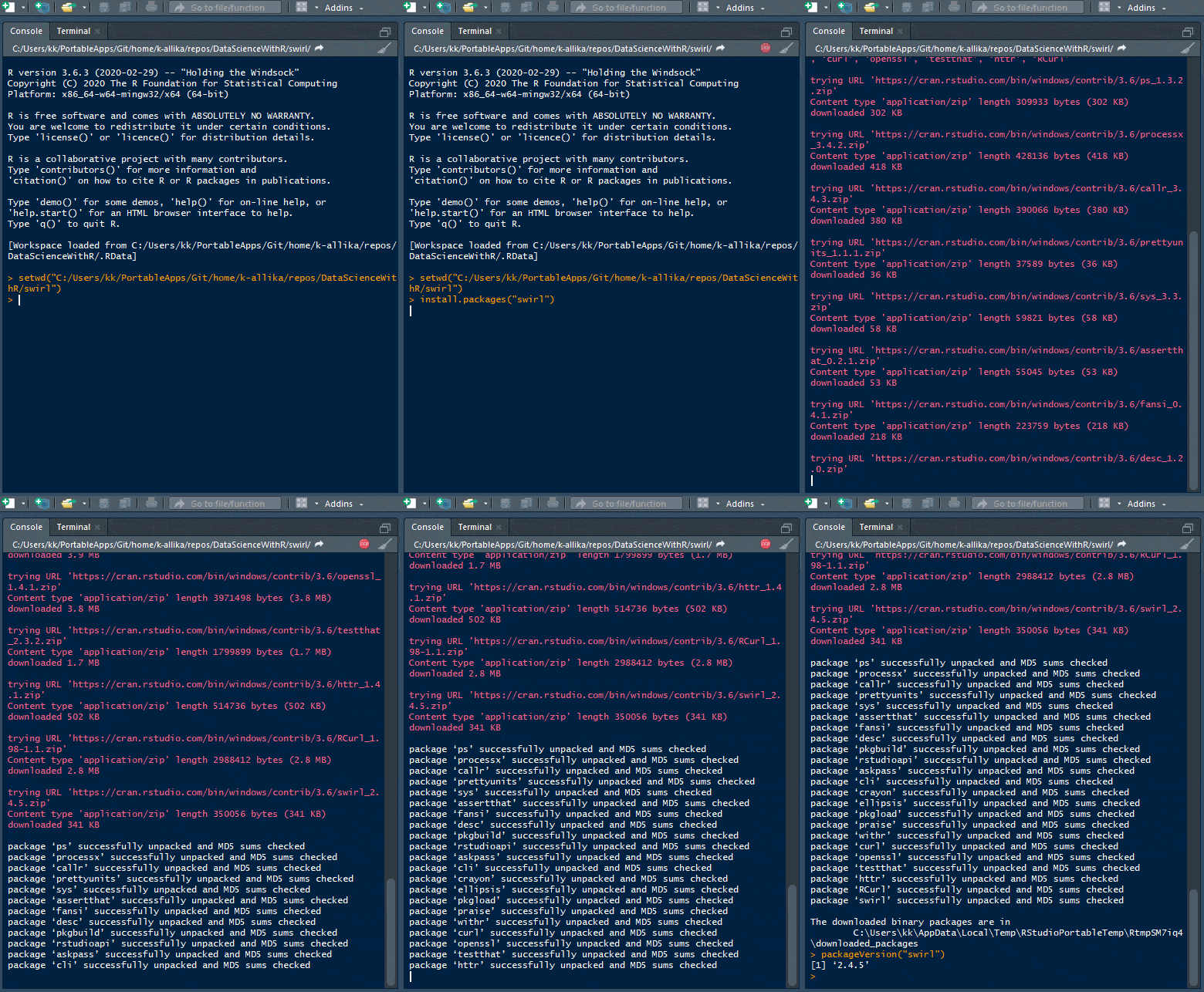
install.packages("swirl")

Check your installation:

packageVersion("swirl")

Installing swirl

[^top]

Installing a course in swirl

Load swirl library.

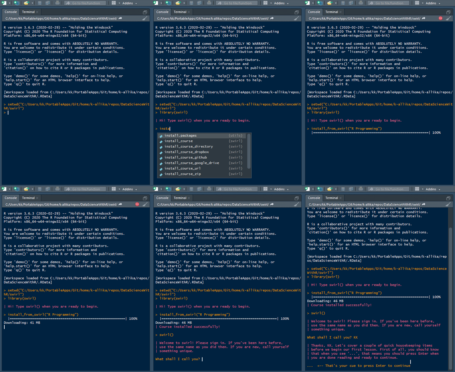
library(swirl)

Install "R Programming" course.

install_from_swirl("R Programming")

Here is a list of all swirl courses http://swirlstats.com/scn/title.html

Installing course

[^top]

Last updated 2020-10-01 18:05:14.907413 IST

Installing R and RStudio

wordcloud

Portable environment

This page will guide you on installing R and RStudio in a portable environment on a Windows 10 system. Following are the reasons why I prefer a portable installation over a regular installation:

  • I am not tied up to a particular computer. Installation and files reside in a portable drive (a pen-drive or a portable hard disk drive). I can use R on any Windows system wherever I go.
  • If this system crashes, I don't lose my setup or files.
  • I like experimenting.

If you prefer a regular installation, visit RStudio and follow the steps.

Installing PortablaApps platform (optional): Portable Apps platforms comes with it's own start menu launcher which is handly when you install multiple portable programs in future. Download and install PortableApps Platform from https://portableapps.com/download.

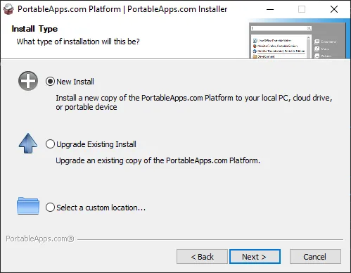
1. Select "New Install" New Install

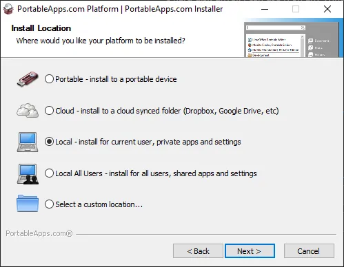
2. Select

  • Portable apps if you want to install it on your pen-drive or a portable hard disk drive
  • Cloud, if you want to intall it in your Dropbox, Google Drive, PCloud, One Drive, etc
  • Local - It will be installed in your local drive but only you can access the programs. Other Windows users on your system will not be able to access your portable applications. This is where I am installing.
  • Local All Users - It will be installed in your local drive and all users on your computer can access them.

Installation options

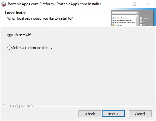
3. Select your preferred directory and continue. Select directory

Once the installation is complete, open Portable Apps platform and if everthing went well, you'll see something like this. PortableApps

[^top]

Installing R

1. Download R Portable paf.exe file from https://sourceforge.net/projects/rportable/.

2. Open PortableApps Menu and go to Apps > Install a New App Install a New App

3. Select the R Portable paf.exe file you downloaded earlier and continue installation with default settings.

4. Once installation is complete, you will be able to see R in your Portable Apps menu. Click on it and open R console. Open R

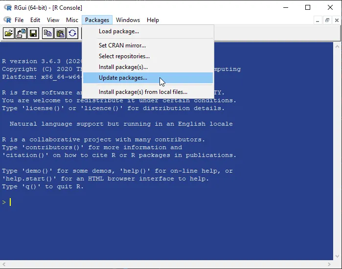
5. Updating R packages: In R Console menu, go to Packages > Update Packages Update Packages

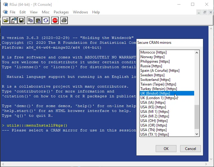
6. Select the CRAN mirror location nearest to you. CRAN mirror location

7. If there are any packages that need to be updated, you'll see a small window with a list of apps selected. Click 'OK' and update them.

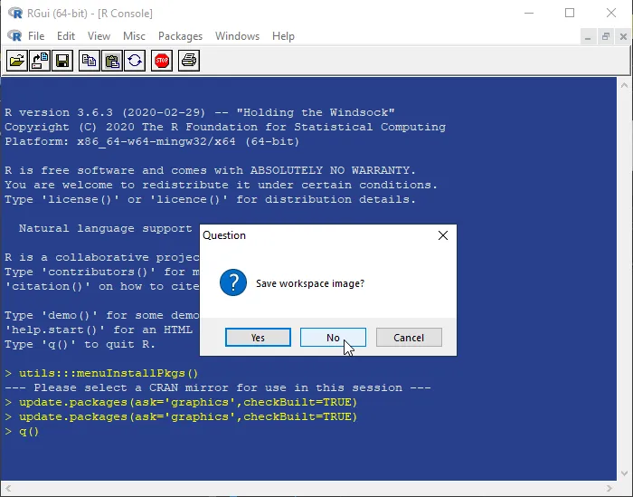
8. Close R console. There is no need to save the workspace image. Close R console

[^top]

Installing RStudio

RStudio is provides the GUI(Graphics User Interface) and is also the commonly used IDE(Integrated Development Environment) for R.

1. Go to https://sourceforge.net/projects/rportable/files/R-Studio/ and select the latest version of RStudio. Download the paf.exe file from the folder.

2. Open PortableApps Menu and go to Apps > Install a New App

3. Select the RStudio Portable paf.exe file you downloaded earlier and continue installation with default settings.

4. Once installation is complete, you will be able to see RStudioPortable in your Portable Apps menu. Click on it and open R Studio.

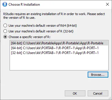
5. The first time you open R Studio, it will ask you to chose the version of R you want to use. select R version

6. Click "Browse" and point to the "bin" directory of portable R you installed earlier. The path looks similar to C:\Users\YourUserName\PortableApps\R-Portable\App\R-Portable\bin.

7. Select 32-bit or 64-bit based on your Windows 10 version. If you are unsure, select 32-bit as it works on both.

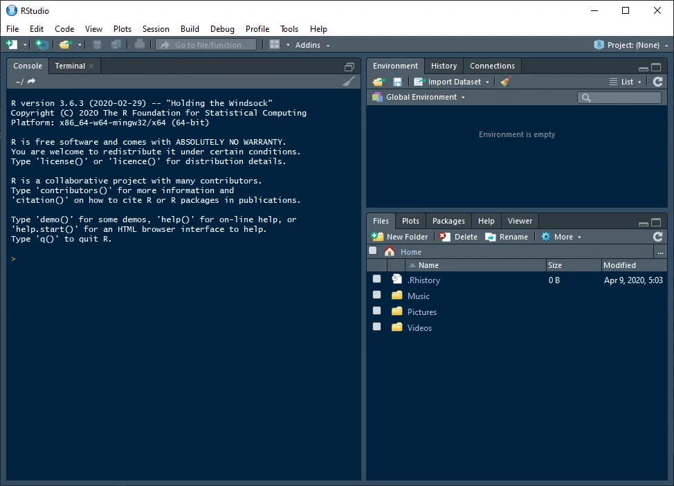
You are now ready to use R Studio. RStudio

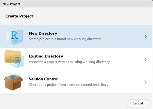
8.\ Create R Project. Select File > New Project. Select "New Directory".

New Directory

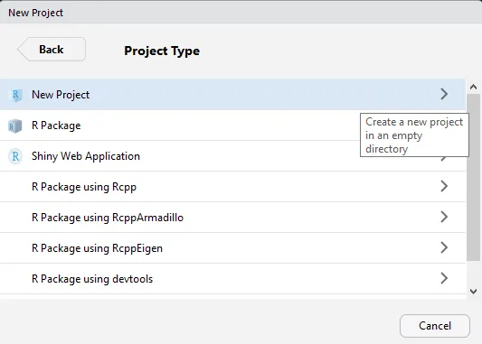
Select "New Project"

New Project

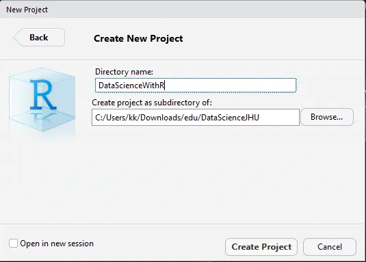
Name your project (example: DataScienceWithR). Browse and select the directory where you want the project to reside. Click "Create Project".

Project name and location

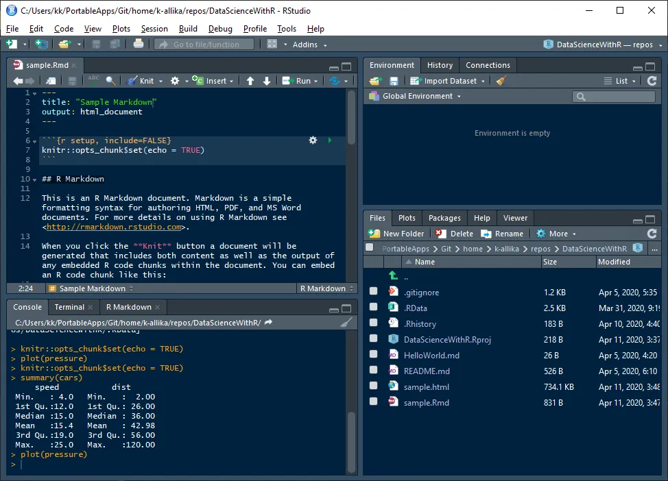
You should now see your project files including "DataScienceWithR.Rproj" file in the second quadrant of R Studio.

[^top]

Installing R Markdown

As a data scientist, it's important to not only write and run code but also explain data manipulation and inferences in words. Markdown allows us to document our work. R-Markdown integrates R code with Markdown to provide an integrated solution. JupyterLab (a successor of iPython) is another such tool, which we will come across soon.

1.\ In R Studio, go to File > New File > R Markdown.

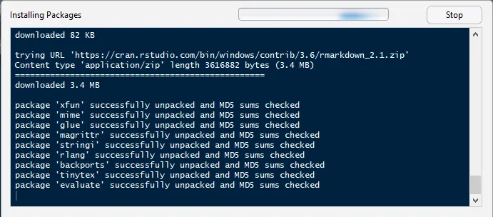
2.\ If there are any missing packages, R Studio will ask you if you'd like to install them. Click 'OK' and wait for it to install.

Installing R Markdown dependencies

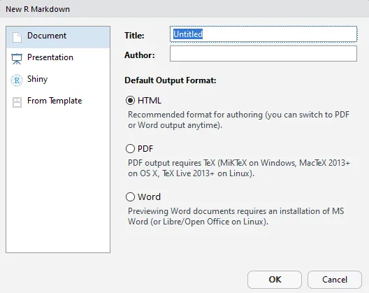
3.\ Give a name to the document (example: sample). Select 'HTML' or 'PDF' as your choice of output.

R Markdown options

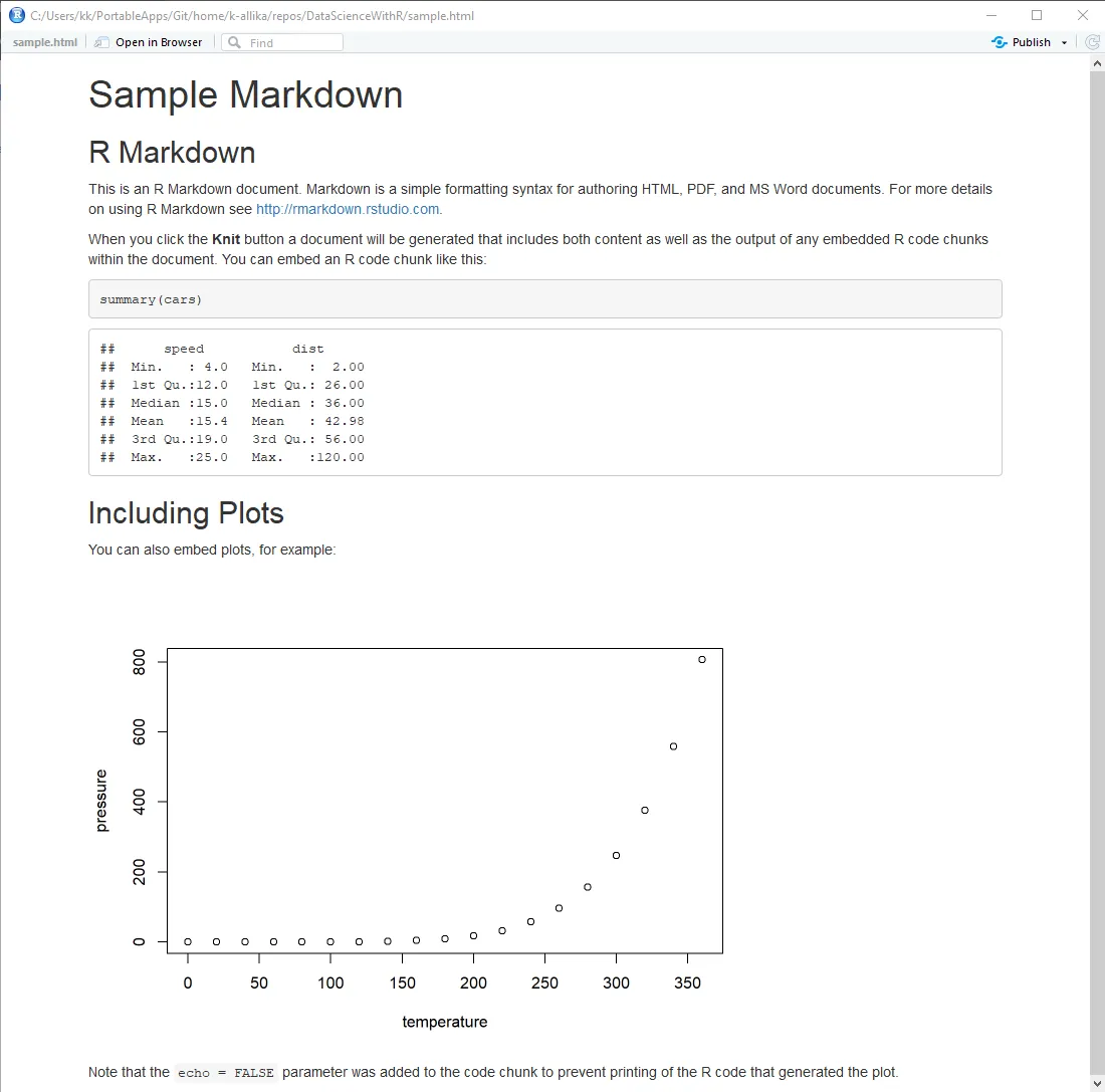
4.\ This will create a sample markdown document with some examples in it. You may change the 'title' in the document to "Sample Markdown". Save the file.

Sample Markdown

5. Press CTRL+SHIFT+K or click the "Knit" button in the fourth quadrant of R Studio or go to File > Knit Document to generate an HTML or PDF output of the markdown file.

HTML output

[^top]

Installing R in JupyterLab (Optional)

This step is completely optional and you can safely skip it. JupyterLab is a web-based interactive development environment for Jupyter notebooks, code, and data. It supports over 40 programming languages including R. I started using JupyterLab a short time ago while learning Python and am quite impressed by its features, interactivity, improvements and its community. This is my attempt to run R in JupyterLab environment.

Follow the steps to install R in JupyterLab. If you already have JupyterLab installed, you can directly go to step x.

1. Anaconda vs Miniconda: To use JupyterLab, you need to have Anaconda or Miniconda installed. Follow either 1a or 1b.

1a. Anaconda comes bundled with Python and a lot of packages commonly used in data science. It also comes with a GUI called Navigator and it's own IDE called Spyder. If you are a beginner, install Anaconda from https://www.anaconda.com/distribution/. Select Python 3+ version. Install will default settings.

1b. Miniconda is a small, bootstrap version of Anaconda that includes only conda, Python, the packages they depend on, and a small number of other useful packages. I prefer Miniconda instead of Anaconda as I don't need Anaconda's GUI and IDE and I am more comfortable with using CLI(Command Line Interface) for installing and maintaining packages. Also, I don't need all the packages that come with Anaconda. I can install the packages I want when I need them. Download Miniconda from https://docs.conda.io/en/latest/miniconda.html. You can install with default settings, or if you prefer a portable version of it, open the command prompt in administrator mode and go to the directory where you downloaded Minoconda exe file and type the following

Miniconda3-latest-Windows-x86_64.exe /InstallationType=JustMe /AddToPath=0 /RegisterPython=0 /NoRegistry=1

2. Creating a virtual environment: In Anaconda(or Miniconda. In future, I am going to use the term Anaconda for both Anaconda and Miniconda because they both have the same core. Whatever works in one, works in the other too.), we have an option to create virtual environments. Each environment can have packages and code specific to its project. This is useful because different projects require different packages and it's not advisable to install all packages at one place in the base(base is the default environment that comes with Anaconda). Also, if you don't want to mess up the base when you are experimenting. Always create a new environment, experiment and if something goes wrong then delete it and create a new one without having to reinstall Anaconda.

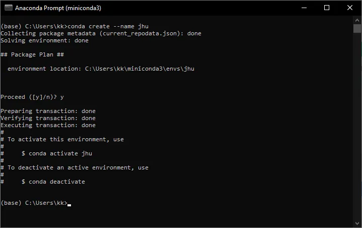
2a. Open 'Anaconda Prompt' from Windows Start Menu

2b. Create a virtual environment. Enter the following in the command prompt.

conda create --name jhu.

I created an environment called 'jhu'. The name is arbitrary. You can name it anything you want.

Create a virtual environment

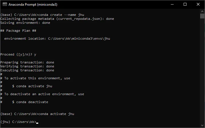
2c. Activate the virtual environment

conda activate jhu

Replace 'jhu' with your environment name. You should see the name of the environment in brackets on the left of the prompt.

Activate the virtual environment

3. Install JupyterLab

conda install -c conda-forge jupyterlab

This will show a list of dependency packages to be installed. Press 'y' and continue.

4. Install R in JupyterLab

4a. Install from R Console: If you already followed the steps above and have successfully installed R in your system, then this is the easiest way to install R in Jupyter Lab.

Open R and enter the following command in R consode window

install.packages("irkernel")

4b. Install from Anaconda prompt: If you don't have R installed in your system and still want to use R in Jupyter Lab, then open Anaconda prompt and enter the following.

conda install -c r r-essentials

This will install R along with essential packages to use R in JupyterLab. Now open JupyterLab by typing the following

jupyter lab

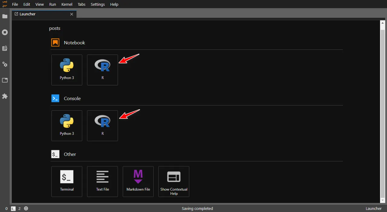
If everywthing went well, you should see JupyterLab launcher with R installed alongside Python.

R kernel in JupyterLab

Let's run a small piece of R code that I copied from here and see if it works.

In [2]:
library(dplyr)
library(ggplot2)
ggplot(data=iris, aes(x=Sepal.Length, y=Sepal.Width, color=Species)) + geom_point(size=3)
No description has been provided for this image

Works well!

[^top]

Last updated 2020-10-01 17:58:31.235073 IST
Introduction to data science

wordcloud

Data science

  • Data science involves statistics, computer science and mathematics.
  • Machine learning and artificial intelligence are two of the most popular branches of data science these days.
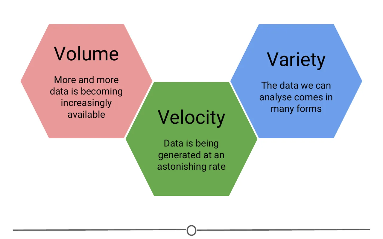
  • Three key features of Big Data
    • Volume - Deals with huge amounts of data.
    • Velocity - Data is generated rapidly, also involves real time data.
    • Variety - Deals with structured and unstructured data.

Three Vs of Big Data

  • A data scientist is someone who applies data science tools to data to answer questions.
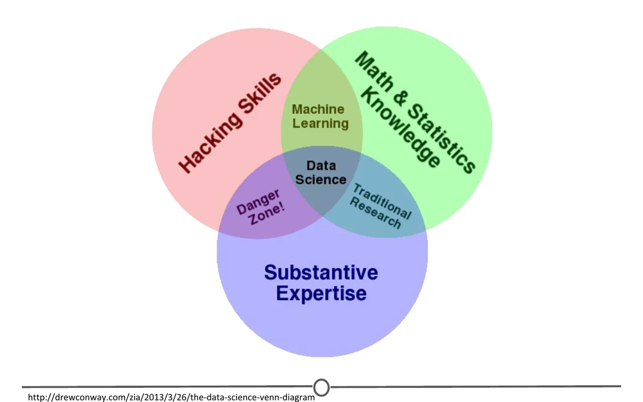
  • Data scientists usually have a combination of the following skills:

Data scientist's skills

[^top]

Data

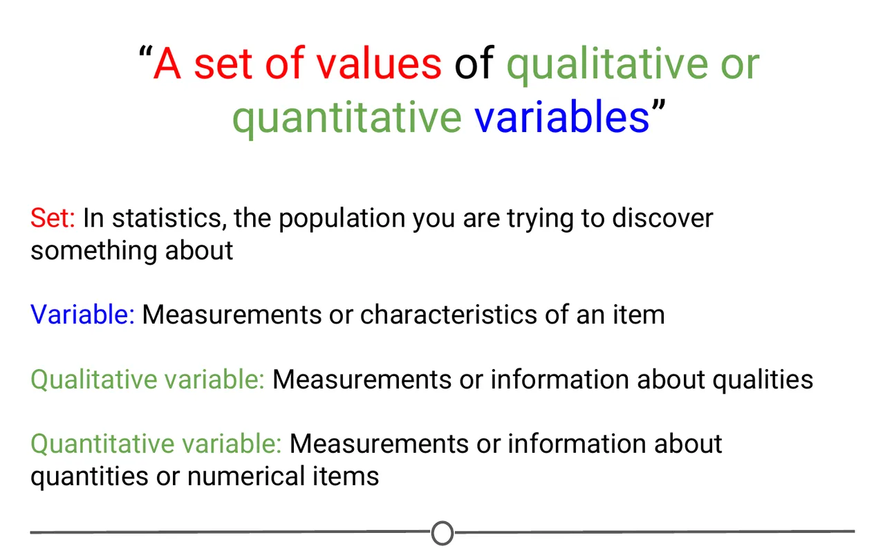
There are several definitions of data. The definition provided by Wikipedia is "A set of values of qualitative or quantitative variables".

Definition of data

There are two kinds of data we usually come across:

  • Structured data - Data that can be stored in tabular format (rows and columns) and each variable (or column) has a specific data type (numeric, text, category, etc)
  • Unstructred data - Any data that is not structured is unstructed data. Some examples are twitter data, facebook comments, sequencing data (medical, genome data), medical records, languages, images, etc

Variables

  • Quantitative - measureable, numeric (integers or real numbers).
    • examples: age, distance, time, etc
  • Qualitative - non-measurable (example: categorical or user assigned)
    • examples: name, severity(High, Medium, Low), ranking, etc
  • Quantitative variables can be discrete or continuous*.

[^top]

Data science project

Steps or life cycle of a data science project

  • Business case (forming a question, scope analysis)
  • Data collection (finding or generating data)
  • Data pruning (data cleansing, data manipulation, data visualization)
  • Data analysis (Exploratory and/or Inferential statistics)
  • Data Modeling (Machine Learning, Artificial Intelligence)
  • Closure (Conclusions, reporting, communication to stakeholders, future scope)

[^top]

* Johns Hopkins University course stated that "Quantitative variables are measured on ordered, continuous scales", which, in my opinion, is a vague statement. Quantitative variables are measured not only on continuous scales but also on discrete (non-continous) scales. Some examples of discrete quantitative variables are 'age in years', 'number of days since first medication', 'number of pencils in a box', etc

Last updated 2020-12-16 16:31:13.188933 IST

GitHub and Git basics

GitHub/GitLab Account

GitHub is a service where you can host your projects online with a lot of free features especially for version control. GitHub is also the most popular Git based online repository service followed by GitLab. Click on the hyperlinks to sign up for a free account.

[^top]

Creating a repository

Login to GitHub and select "New Repository". Give a name to your repository(also called repo). Select option "Public" or "Private" depending on whether you want to share your repo with others or not.

[^top]

Installing Git

Download and install Git for Windows from https://git-scm.com/download/win. You can install the regular version or the portable version of from the links on the page. By now, you might have guesed that I have installed the portable version.

[^top]

Connecting R Studio to GitHub

JHU's Linking GitHub and RStudio document shows in detail how to connect R Studio to your GitHub account, create projects in repositories, commit and push repos. Hence, I am not going to go through that here. Also, I am not a big fan of using R Studio to perform Git operations. I believe that one needs to work on CLIs (like Git Bash) to learn and understand how Git versioning works.

[^top]

Git Bash

Git Bash is a CLI(Command Line Interface) for Git operations for Git based online services like GitHub or GitLab. We have already installed Git earlier which contains an executable file called Git Bash. We will use Git Bash to connect to GitHub and perform Git operations.

1. Git Credential Manager for Windows (GCMW)

Git Bash can connect to Github via SSH or HTTPS. GitHub recommends HTTPS over SSH as the connections are much faster and easier to set up. To connect over HTTPS, we need to install Git Credential Manager for Windows (GCMW). GCMW provides secure Git credential storage for Windows with Two-factor authentication for GitHub. Download and install the latest GCMW from https://github.com/Microsoft/Git-Credential-Manager-for-Windows/releases/latest

2. Git Bash first time configuration

Here are a few things that you need to do when you first install Git. Open Git Bash and you'll see a CLI that looks like this.

Git Bash

1. Type the following command in Git Bash and enter your GitHub username (the one created while setting up the GitHub account) in quotes.

git config --global user.name "YourUserName"

2. Enter your email address associated with your GitHub account.

git config --global user.email [email protected]

3. Configure your favorite text editor for Git Bash. If you installed portable Notepad++ like me, you can configure it as your default Git Bash text editor by typing the following. Edit Notepad++ path accordingly.

git config --global core.editor "'C:/Users/kk/PortableApps/Notepad++Portable/App/Notepad++/notepad++.exe' -multiInst -notabbar -nosession -noPlugin"

You can also check your settings by entering the following. If something's wrong, use the above commands to change them.

git config --list

Git config

3. Basic Git operations

Let's create a repository called "testrepo" and perform some basic Git operations on it. Login to GitHub and create the repository called "testrepo".

Create repo

Ensure that the connection is HTTPS. Click copy button to copy the repo link.

Copy repo link

Go to Git Bash and create a directory where you plan to work on your projects. Let's call it "projects".

mkdir projects

Enter the following command to view all files and directories in the current location. One of them should read "projects"

Change directory to "projects"

cd projects

git clone

Clone your repo to your current working directory.

git clone https://github.com/k-allika/testrepo.git

git remote

Check connection to your remote repo

git remote -v

.gitignore

.gitignore is an important file and should be created before the first push. .gitignore contains a list of files that git will ignore while performing git operations. For example, if I have some text files in my working directory that I do not want to push them to my GitHub repo, then I'll include *.txt in my .gitignore.

touch

Create an empty .gitignore file

touch .gitignore

vi

Edit an existing file or create a new file and edit.

vi .gitignore

adding *.txt to ignore will tell Git to ignore all txt files and not to push them to remote repo.

Basic vi commands:

i to start editing.

Esc to stop editing and come out of edit mode.

:w to save file.

:q to quit vi

Let's create a "notes.txt" file to test .gitignore. Since we added *.txt to .gitignore, "notes.txt" would not be pushed to the repo.

vi notes.txt

Let's create another file called "README.md". Since this file does not match anything in .gitignore, it would be pushed to the repo.

vi README.md

ls

ls lists files and directories in the current directory. The arguments -la will show file attributes along with hidden files.

ls -la

git status

View the status of your working directory compared to the remote repo at GitHub.

git status

As expected, you'll notice that only .gitignore and README.md files are mentioned in the status output. The notes.txt is ignore as it should.

git push

git push

Push changes in your working directory to the remote repo.

Git Bash Basics

Check your repo at GitHub and you should see the changes there.

Remote repo

[^top]

Last updated 2020-04-13 22:32:36.916238 IST

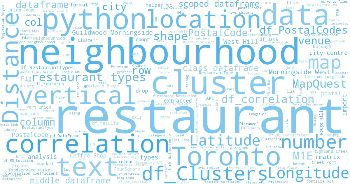
Insights into Toronto’s Foodservice Market

wordcloud

Podcast

Give your eyes a break—listen to my article instead!

Abstract

The project delivers valuable decision driven insights into Toronto's foodservice industry by employing modern-day data science tools. K means, an unsupervised clustering algorithm is applied to segregate the city's restaurant market into clusters based on the types of restaurants established in the city. Relationship between foodservice market of a neighbourhood and its location relative to the city centre along with relationships within various types of restaurants are analysed using inferential statistics.

Introduction/Business Understanding

Background

By 2022, quick-service restaurants are expected to remain the largest segment in the foodservice industry in Canada followed by full-service restaurants. However, Toronto’s landscape is unique compared to the rest of the country. Toronto has comparatively higher percentages of coffee shops and fine dining restaurants compared to the national average. There are also more restaurants serving European menus in Toronto than in other places, whereas the “hamburger” type menus are relatively scarce in the city. It is interesting to note that Toronto has a very strong presence of independently owned restaurants making up more than 90% of the city’s foodservice market.

Area of Interest

With a blooming foodservice market, Toronto constantly attracts new restaurants and eateries. The target audience of the project are the investors and potential restaurant owners are often faced with several market research questions such as the current market landscape in the area of interest, the type of restaurant that fits well with the neighbourhood, the best location for a particular type of restaurant, etc. However, since Toronto's foodservice market is unique to itself, new owners cannot simply rely on a nationwide analysis. A city-specific analysis is what would benefit anyone who intends to start a new restaurant in Toronto and that is precisely what this project presents.

Problem Statement

This project aims to provide valuable insights into Toronto’s current foodservice market such as distribution of restaurant types by locations, variations in density of restaurants and suggestive analysis of types of restaurants to benefit new and potential restaurant owners and investors.

Analytical Approach

Clustering

The approach is to categorize types of restaurants in Toronto into various clusters and map them to their geographical locations. A visualization map of Toronto would illustrate these clusters cast across its postal codes.

Correlation

Further analysis is done to identify any correlation between restaurants in the neighbourhood and its distance from the city centre, and any significant correlations within types of restaurants.

Data Acquisition

Data requirements

The data required for the project includes the list of postal codes of the city, types of restaurants in each location, number of restaurants of each type, distances of restaurants from the city centre, and the geographical coordinates of the postal codes to visualize the data in a map.

Data collection

Neighbourhood data

Postal code data for Toronto is scraped from the following Wikipedia page:

Source: https://en.wikipedia.org/wiki/List_of_postal_codes_of_Canada:_M

Data points:

  • Postal code

  • Borough

  • Neighbourhood

Geographical coordinates

Geographical coordinates data is extracted using Mapquest’s Geocoding API:

Source: https://developer.mapquest.com/documentation/geocoding-api/

Alternate source (Google API): https://link.datascience.eu.org/p001d1

Data points:

  • Postal code

  • Latitude

  • Longitude

Foodservice market data

Restaurant data is extracted from FourSquare’s Places API. FourSquare data is classified into various categories and sub-categories. Categories are identified by the tag "Category ID". The category of interest here is Food and the category ID for food is 4d4b7105d754a06374d81259. The sub-categories of the food category are various types of restaurants located in the venue.

Source: https://developer.foursquare.com/docs/api/endpoints

Data points:

  • Postal code

  • Venue Latitude

  • Venue Longitude

  • Venue category

  • Venue subcategory

Table 1. Data points and data sources.

Datapoint Source
Postal Code Wikipedia
Borough Wikipedia
Neighbourhood Wikipedia
Postal Code MapQuest Geocoding API
Latitude MapQuest Geocoding API
Longitude MapQuest Geocoding API
Postal Code FourSquare Places API
Venue Latitude FourSquare Places API
Venue Longitude FourSquare Places API
Venue Category FourSquare Places API
Venue Subcategory FourSquare Places API

Code for data collection

Importing libraries

In [1]:
import numpy as np  # Numpy library
import pandas as pd  # library for data analysis
import json  # library to handle JSON files
import geocoder  # convert an address into latitude and longitude values
from geopy.geocoders import Nominatim  # convert an address into latitude and longitude values
import requests  # library to handle requests
import matplotlib.cm as cm  # Matplotlib and associated plotting modules
import matplotlib.colors as colors
import matplotlib.pyplot as plt
from sklearn.cluster import KMeans  # import k-means from clustering stage
import folium  # map rendering library
import seaborn as sns  # Seaborn
from scipy.stats import pearsonr  # Pearson correlation library
from getpass import getpass as gp  # to hide API keys from being displayed
from tabulate import tabulate  # to pretty print tabular data
In [2]:
pd.set_option('display.max_columns', 10)
pd.set_option('display.max_rows', 10)

Scraping neighbourhood data from the web

Since the neighbourhood and postal code data is already in the form of a table, we can use the pandas read_html which looks for tabular data and loads it into a data frame

In [2]:
df_PostalCodes = \
    pd.read_html('https://en.wikipedia.org/wiki/List_of_postal_codes_of_Canada:_M'
                 )[0]

Collecting geographical coordinates from MapQuest

Documentation for MapQuest Geocoding API is available at https://geocoder.readthedocs.io/providers/MapQuest.html

In [4]:
MapQuest_key = gp("Enter your MapQuest API key")
In [39]:
# Collecting coordinates from MapQuest geocode API for a sample of 5 postal codes.

sample = 5
df_MQ_Coordinates = pd.DataFrame(columns=['Latitude', 'Longitude'])
for i in range(sample):
    g = geocoder.mapquest(df_PostalCodes.loc[i, 'Postcode']
                          + ', Toronto, Ontario', key=MapQuest_key)
    df_MQ_Coordinates.loc[i] = g.latlng

Extracting types of restaurants from FourSquare

FourSquare's category ID for Food is 4d4b7105d754a06374d81259. Venues will be searched in each neighbourhood by this category ID. The restaurant type, which is the sub-category, of each venue is extracted. If there are no restaurants in a neighbourhood, then the restaurant type will be assigned as "No Restaurants".

In [34]:
FourSquare_client_ID = gp('Enter your FourSquare Client ID')
FourSquare_client_secret = gp('Enter your FourSquare Client Secret')
FourSquare_API_version = '20190801'  # Foursquare API version
In [40]:
# Extracting restaurant data for a sample of 5 locations

df_MQ_Location = pd.concat([df_PostalCodes.head(sample),
                           df_MQ_Coordinates], axis=1)
df_RestaurantTypes = pd.DataFrame(columns=['RestaurantType',
                                  'PostalCode'])
for (index, row) in df_MQ_Location.iterrows():
    limit = 100  # limit of number of venues returned by Foursquare API
    radius = 300  # define radius
    cat_id = '4d4b7105d754a06374d81259'  # Category: Food
    url = 'https://api.foursquare.com/v2/venues/search?&client_id={}&client_secret={}&v={}&ll={},{}&radius={}&limit={}&categoryId={}'.format(
        FourSquare_client_ID,
        FourSquare_client_secret,
        FourSquare_API_version,
        row['Latitude'],
        row['Longitude'],
        radius,
        limit,
        cat_id,
        )
    df_results = pd.DataFrame(list(venue['categories'][0]['name']
                              for venue in
                              requests.get(url).json()['response']['venues']), columns=['RestaurantType'])
    if df_results.shape[0] == 0:
        df_results.loc[0, ['RestaurantType']] = 'No Restaurants'
    df_results['PostalCode'] = row['Postcode']
    df_RestaurantTypes = pd.concat([df_RestaurantTypes, df_results])
df_RestaurantTypes.reset_index(drop=True, inplace=True)

Data Preparation and Feature Extraction

Data understanding

In [41]:
# Checking neighbourhood data

print('Shape:', df_PostalCodes.shape)
df_PostalCodes.head()
Shape: (288, 3)
Out[41]:
Postcode Borough Neighbourhood
0 M1A Not assigned Not assigned
1 M2A Not assigned Not assigned
2 M3A North York Parkwoods
3 M4A North York Victoria Village
4 M5A Downtown Toronto Harbourfront

The neighbourhood data contains the variables Postcode, Borough and Neighbourhood.

In [42]:
# Checking geographical coordinates data

print('Shape:', df_MQ_Coordinates.shape)
df_MQ_Coordinates.head()
Shape: (5, 2)
Out[42]:
Latitude Longitude
0 43.63175 -79.41944
1 43.63175 -79.41944
2 43.76523 -79.33701
3 43.73279 -79.31051
4 43.65331 -79.36646

The geographical data from MapQuest contains variables PostalCode, Latitude and Longitude.

In [43]:
df_RestaurantTypes.head()
Out[43]:
RestaurantType PostalCode
0 Food Truck M1A
1 Poutine Place M1A
2 Fast Food Restaurant M1A
3 Wings Joint M1A
4 Donut Shop M1A

The FourSquare API data contains records of variables RestaurantType and PostalCode.

Data Preperation

Postal code and neighbourhood data

In [3]:
# Renaming column names

df_PostalCodes.rename(columns={'Postcode': 'PostalCode'}, inplace=True)

# Ignore cells with a borough that is 'Not assigned'

df_PostalCodes = df_PostalCodes.query("Borough != 'Not assigned'"
        ).reset_index(drop=True)

# Combining neighbourhoods belonging to same postal code

df_PostalCodes = df_PostalCodes.groupby('PostalCode',
        as_index=False).agg(lambda x: ', '.join(sorted(set(x))))

# Assigning borough names to 'Not assigned' neighbourhoods

df_PostalCodes.loc[df_PostalCodes['Neighbourhood'] == 'Not assigned',
                   'Neighbourhood'] = df_PostalCodes['Borough']
df_PostalCodes.head(5)
Out[3]:
PostalCode Borough Neighbourhood
0 M1B Scarborough Malvern, Rouge
1 M1C Scarborough Highland Creek, Port Union, Rouge Hill
2 M1E Scarborough Guildwood, Morningside, West Hill
3 M1G Scarborough Woburn
4 M1H Scarborough Cedarbrae
In [56]:
print('Shape:', df_PostalCodes.shape)
Shape: (103, 3)

The extracted data contains numerous issues that were fixed. The neighbourhood data contained postal codes without any boroughs assigned which were dropped. Some neighbourhoods were not assigned a neighbourhood name, so their borough names were assigned to them. In some cases, more than one neighbourhood shared the same postal code. After fixing these issues, the data contained 103 records of postal code data.

In [22]:
# Extracting coordinates data from MapQuest API

df_MQ_Coordinates = pd.DataFrame(columns=['Latitude', 'Longitude'])
for i in range(df_PostalCodes.shape[0]):
    g = geocoder.mapquest(df_PostalCodes.loc[i, 'PostalCode']
                          + ', Toronto, Ontario', key=MapQuest_key)
    df_MQ_Coordinates.loc[i] = g.latlng

Plotting a map of neighbourhoods with MapQuest data

In [4]:
address = 'Toronto, Ontario'
geolocator = Nominatim(user_agent='my-application')
location = geolocator.geocode(address)
latitude = location.latitude
longitude = location.longitude
print('The geograpical coordinates of Toronto, Ontario are {}, {}.'.format(latitude,
        longitude))
The geograpical coordinates of Toronto, Ontario are 43.653963, -79.387207.
In [24]:
df_MQ_Location = pd.concat([df_PostalCodes, df_MQ_Coordinates], axis=1)
map_Toronto_MapQuest = folium.Map(location=[latitude + 0.07,
                                  longitude], zoom_start=11)  # Offset to centre the map around neighbourhoods

# add markers to the map

for (lat, lon, pc, nbh) in zip(df_MQ_Location['Latitude'],
                               df_MQ_Location['Longitude'],
                               df_MQ_Location['PostalCode'],
                               df_MQ_Location['Neighbourhood']):
    label = folium.Popup('{}: {}'.format(pc, nbh), parse_html=True)

    folium.CircleMarker(
        [lat, lon],
        radius=5,
        popup=label,
        color='blue',
        fill=True,
        fill_color='#3186cc',
        fill_opacity=0.7,
        parse_html=False,
        ).add_to(map_Toronto_MapQuest)
map_Toronto_MapQuest
Out[24]:

Fig 01. Toronto neighbourhood map using MapQuest API coordinates

The geographical coordinates data extracted from MapQuest had some concerns too. The postal code data is merged with the coordinates and plotted on a map to get a basic understanding of the data. Following image displays a map of Toronto with neighbourhood markers overlayed on it. It was observed that the MapQuest latitude and longitude were not accurate and many of the nearby neighbourhoods had the same coordinates.

So the coordinates data is replaced by the data extracted from the alternate source, a static CSV file of Google API output. The following image displays a map of Toronto with the neighbourhoods as markers. The latitude of the map is offset by 0.07 to centre the map around the neighbourhoods.

Plotting a map of neighbourhoods with the CSV data from Google API

In [5]:
df_csv_Coordinates = pd.read_csv('http://link.datascience.eu.org/p001d1')
df_csv_Coordinates.rename(columns={'Postal Code': 'PostalCode'},
                          inplace=True)
df_csv_Location = pd.merge(df_PostalCodes, df_csv_Coordinates,
                           on='PostalCode')
In [8]:
map_Toronto_CSV = folium.Map(location=[latitude + 0.07, longitude],
                             zoom_start=11)

# add markers to the map

for (lat, lon, pc, nbh) in zip(df_csv_Location['Latitude'],
                               df_csv_Location['Longitude'],
                               df_csv_Location['PostalCode'],
                               df_csv_Location['Neighbourhood']):
    label = folium.Popup('{}: {}'.format(pc, nbh), parse_html=True)

    folium.CircleMarker(
        [lat, lon],
        radius=5,
        popup=label,
        color='blue',
        fill=True,
        fill_color='#3186cc',
        fill_opacity=0.7,
        parse_html=False,
        ).add_to(map_Toronto_CSV)
map_Toronto_CSV
Out[8]:

Fig 02. Toronto neighbourhood map using Google API coordinates

Examining the maps above, it is evident that the coordinates data from Google API is of better quality than that of MapQuest. Hence, the MapQuest data is discarded and Google coordinates data is used.

In [58]:
df_Location = df_csv_Location.drop(['Borough'], axis=1)
df_Location.head()
Out[58]:
PostalCode Neighbourhood Latitude Longitude
0 M1B Malvern, Rouge 43.806686 -79.194353
1 M1C Highland Creek, Port Union, Rouge Hill 43.784535 -79.160497
2 M1E Guildwood, Morningside, West Hill 43.763573 -79.188711
3 M1G Woburn 43.770992 -79.216917
4 M1H Cedarbrae 43.773136 -79.239476

FourSquare Restaurant data

In [59]:
df_RestaurantTypes = pd.DataFrame(columns=['RestaurantType',
                                  'PostalCode'])
for (index, row) in df_Location.iterrows():
    limit = 100  # limit of number of venues returned by Foursquare API
    radius = 300  # define radius
    cat_id = '4d4b7105d754a06374d81259'  # Category: Food
    url = \
        'https://api.foursquare.com/v2/venues/search?&client_id={}&client_secret={}&v={}&ll={},{}&radius={}&limit={}&categoryId={}'.format(
        FourSquare_client_ID,
        FourSquare_client_secret,
        FourSquare_API_version,
        row['Latitude'],
        row['Longitude'],
        radius,
        limit,
        cat_id,
        )
    df_results = pd.DataFrame(list(venue['categories'][0]['name']
                              for venue in
                              requests.get(url).json()['response'
                              ]['venues']), columns=['RestaurantType'])
    if df_results.shape[0] == 0:
        df_results.loc[0, ['RestaurantType']] = 'No Restaurants'
    df_results['PostalCode'] = row['PostalCode']
    df_RestaurantTypes = pd.concat([df_RestaurantTypes, df_results])
df_RestaurantTypes.reset_index(drop=True, inplace=True)
In [60]:
# Checking FourSquare data

print('Shape:', df_RestaurantTypes.shape)
df_RestaurantTypes.head()
Shape: (1567, 2)
Out[60]:
RestaurantType PostalCode
0 No Restaurants M1B
1 No Restaurants M1C
2 Restaurant M1E
3 Bakery M1E
4 Chinese Restaurant M1E

The FourSquare API returned 1564 records of variables RestaurantType and PostalCode, of which, some locations did not have any restaurants within the specified radius. The RestaurantType variable for such locations was marked as No Restaurants.

Feature Extraction

In [61]:
df_Data = pd.merge(df_Location, df_RestaurantTypes, on='PostalCode')
df_Data.head()
Out[61]:
PostalCode Neighbourhood Latitude Longitude RestaurantType
0 M1B Malvern, Rouge 43.806686 -79.194353 No Restaurants
1 M1C Highland Creek, Port Union, Rouge Hill 43.784535 -79.160497 No Restaurants
2 M1E Guildwood, Morningside, West Hill 43.763573 -79.188711 Restaurant
3 M1E Guildwood, Morningside, West Hill 43.763573 -79.188711 Bakery
4 M1E Guildwood, Morningside, West Hill 43.763573 -79.188711 Chinese Restaurant

Along with the extracted features such as PostalCode, Neighbourhood, Latitude, Longitude and RestaurantType, a new variable for the distance of the location from the city centre is added as Distance.

The Distance of a location x1 from the city centre x is calculated using the famous Pythagoras theorem. However, latitudes and longitudes do not follow the same scale throughout the globe. The distance between any two consecutive latitudes is 111 kilometres, but the distance between two consecutive longitudes varies depending on where on Earth we are measuring it. The distance between two longitudes at the Equator is 111 kilometres but it gradually decreases as we move away from the Equator and toward the poles. The information at the National Oceanic and Atmospheric Administration website is used to calculate the approximate distance between two consecutive longitudes in Toronto to be 80 kilometres. The following image illustrates the calculation of the distance of a location from Toronto city centre.

Fig 03. Distance of a location from city centre using Pythagoras theorem

In [62]:
# Distance between two consecutive longitudes in Toronto in kilometers
dLng = 80
# Distance between two consecutive latitudes in kilometers
dLat = 111
df_Data.insert(4, 'Distance', (((df_Data['Longitude'] - longitude)
               * dLng) ** 2 + ((df_Data['Latitude'] - latitude) * dLat)
               ** 2) ** 0.5)
df_Data.head()
Out[62]:
PostalCode Neighbourhood Latitude Longitude Distance RestaurantType
0 M1B Malvern, Rouge 43.806686 -79.194353 22.921869 No Restaurants
1 M1C Highland Creek, Port Union, Rouge Hill 43.784535 -79.160497 23.216478 No Restaurants
2 M1E Guildwood, Morningside, West Hill 43.763573 -79.188711 20.004767 Restaurant
3 M1E Guildwood, Morningside, West Hill 43.763573 -79.188711 20.004767 Bakery
4 M1E Guildwood, Morningside, West Hill 43.763573 -79.188711 20.004767 Chinese Restaurant

Following are the extracted and calculated features of the data frame df_Data used in the analysis.

Feature Source Description Purpose
PostalCode Extracted from Wikipedia A three-letter alphanumeric postcode of a neighbourhood in Toronto Primary key to merge various data frames.
Neighbourhood Extracted from Wikipedia One or more neighbourhood names that fall within the area of the postcode. A key variable around which the analysis is done. Also used as markers on the map.
Latitude Extracted from MapQuest or Google API Latitude of the postcode in decimal units. To locate neighbourhoods on the map and to calculate the distance of a location from the city centre.
Longitude Extracted from MapQuest or Google API Longitude of the postcode in decimal units. To locate neighbourhoods on the map and to calculate the distance of a location from the city centre.
Distance Calculated Distance of a location from the city centre in kilometres. To calculate the correlation between the distance of a location from the city centre and the number of restaurants in the location.
RestaurantType Extracted from FourSquare API Type of a restaurant. To partition the city of Toronto into various clusters based on restaurant types located in the city. Also used to find possible correlations between various restaurant types within the city.
In [82]:
# Run this code if you are not using FourSquare API
# A copy of df_Data data frame is available for download
# from https://link.datascience.eu.org/p001d2

df_Data = pd.read_csv('http://link.datascience.eu.org/p001d2', encoding='utf-8')
df_Data.head()
Out[82]:
PostalCode Neighbourhood Latitude Longitude Distance RestaurantType
0 M1B Malvern, Rouge 43.806686 -79.194353 22.921869 No Restaurants
1 M1C Highland Creek, Port Union, Rouge Hill 43.784535 -79.160497 23.216478 No Restaurants
2 M1E Guildwood, Morningside, West Hill 43.763573 -79.188711 20.004767 Bakery
3 M1E Guildwood, Morningside, West Hill 43.763573 -79.188711 20.004767 Restaurant
4 M1E Guildwood, Morningside, West Hill 43.763573 -79.188711 20.004767 Chinese Restaurant

Exploratory Data Analysis - Clustering Toronto neighbourhoods by restaurant types

K-Means Clustering

Clustering or cluster analysis is the process of dividing data into groups (clusters) in such a way that objects in the same cluster are more similar to each other than those in other clusters. The goal is to divide Toronto neighbourhoods into various groups based on the top 10 types of restaurants located in the neighbourhoods. There are various models and techniques for cluster analysis. K-means clustering is a simple unsupervised learning algorithm that is commonly used for market segmentation. The RestaurantType column is first one-hot encoded and grouped by PostalCode.

One-hot encoding and grouping by postal codes

In [72]:
df_Clusters = df_Data.copy()

# df_OneHot = pd.get_dummies(df_Clusters[["RestaurantType"]], prefix="", prefix_sep="", drop_first=True)

df_Clusters = df_Clusters.drop('RestaurantType',
                               axis=1).join(pd.get_dummies(df_Clusters[['RestaurantType'
        ]], prefix='', prefix_sep=''))
print(df_Clusters.shape)
df_Clusters.head(5)
(1564, 125)
Out[72]:
PostalCode Neighbourhood Latitude Longitude Distance ... Turkish Restaurant Vegetarian / Vegan Restaurant Vietnamese Restaurant Wine Bar Wings Joint
0 M1B Malvern, Rouge 43.806686 -79.194353 22.921869 ... 0 0 0 0 0
1 M1C Highland Creek, Port Union, Rouge Hill 43.784535 -79.160497 23.216478 ... 0 0 0 0 0
2 M1E Guildwood, Morningside, West Hill 43.763573 -79.188711 20.004767 ... 0 0 0 0 0
3 M1E Guildwood, Morningside, West Hill 43.763573 -79.188711 20.004767 ... 0 0 0 0 0
4 M1E Guildwood, Morningside, West Hill 43.763573 -79.188711 20.004767 ... 0 0 0 0 0

5 rows × 125 columns

In [73]:
df_Clusters = df_Clusters.groupby(['PostalCode', 'Neighbourhood',
                                  'Latitude', 'Longitude', 'Distance'
                                  ]).sum().reset_index()
print(df_Clusters.shape)
df_Clusters.head()
(103, 125)
Out[73]:
PostalCode Neighbourhood Latitude Longitude Distance ... Turkish Restaurant Vegetarian / Vegan Restaurant Vietnamese Restaurant Wine Bar Wings Joint
0 M1B Malvern, Rouge 43.806686 -79.194353 22.921869 ... 0 0 0 0 0
1 M1C Highland Creek, Port Union, Rouge Hill 43.784535 -79.160497 23.216478 ... 0 0 0 0 0
2 M1E Guildwood, Morningside, West Hill 43.763573 -79.188711 20.004767 ... 0 0 0 0 0
3 M1G Woburn 43.770992 -79.216917 18.823836 ... 0 0 0 0 0
4 M1H Cedarbrae 43.773136 -79.239476 17.738704 ... 0 0 0 0 0

5 rows × 125 columns

Following are the top 10 types of restaurants in Toronto

In [74]:
top_count = 10  # Number of top restaurant types
top_restaurant_types = df_Clusters[list(df_Clusters.iloc[:, 5:
                                   ])].sum(axis=0).reset_index().sort_values(by=0,
        ascending=False).iloc[:top_count]['index'].values.tolist()
print(tabulate(pd.DataFrame({'Top 10 restaurant types': top_restaurant_types}).set_index('Top 10 restaurant types'
               ), headers='keys', tablefmt='psql'))
+---------------------------+
| Top 10 restaurant types   |
|---------------------------|
| Coffee Shop               |
| Café                      |
| Restaurant                |
| Pizza Place               |
| Fast Food Restaurant      |
| Italian Restaurant        |
| Sandwich Place            |
| Bakery                    |
| Sushi Restaurant          |
| Breakfast Spot            |
+---------------------------+

Determining the optimal k

In [75]:
# Determining optimal k

df_kmeans = df_Clusters[top_restaurant_types]
distortions = []
K = range(1, 10)
for k in K:
    kmeans = KMeans(n_clusters=k, random_state=3).fit(df_kmeans)
    distortions.append(kmeans.inertia_)
plt.plot(K, distortions, 'bx-')
plt.xlabel('k')
plt.ylabel('Distortion')
plt.title('Fig 04. The Elbow method showing the optimal k')
plt.show()
No description has been provided for this image

The optimal value of the number of clusters, k, is determined using the elbow method to be 3.

In [76]:
k = 3  # Number of clusters
kmeans = KMeans(n_clusters=k, random_state=3).fit(df_kmeans)
# df_Clusters.insert(2, 'Cluster', kmeans.labels_)
df_Clusters['Cluster']=kmeans.labels_
df_Clusters.head(5)
Out[76]:
PostalCode Neighbourhood Latitude Longitude Distance ... Vegetarian / Vegan Restaurant Vietnamese Restaurant Wine Bar Wings Joint Cluster
0 M1B Malvern, Rouge 43.806686 -79.194353 22.921869 ... 0 0 0 0 0
1 M1C Highland Creek, Port Union, Rouge Hill 43.784535 -79.160497 23.216478 ... 0 0 0 0 0
2 M1E Guildwood, Morningside, West Hill 43.763573 -79.188711 20.004767 ... 0 0 0 0 0
3 M1G Woburn 43.770992 -79.216917 18.823836 ... 0 0 0 0 0
4 M1H Cedarbrae 43.773136 -79.239476 17.738704 ... 0 0 0 0 0

5 rows × 126 columns

The neighbourhoods are grouped into three clusters. The following table shows the cluster number and the number of neighbourhoods in each cluster.

In [77]:
# Pretty-printing clusters in tabular format.

print(tabulate(df_Clusters['Cluster'
               ].value_counts().sort_index().to_frame(),
               headers=['Cluster number',
               'Neighbourhoods in the cluster'], tablefmt='psql',
               colalign=('center', 'center')))
+------------------+---------------------------------+
|  Cluster number  |  Neighbourhoods in the cluster  |
|------------------+---------------------------------|
|        0         |               79                |
|        1         |               13                |
|        2         |               11                |
+------------------+---------------------------------+
In [79]:
# This code is optional
# A copy of df_Clusters is available for download
# at https://link.datascience.eu.org/p001d3

df_Clusters = pd.read_csv('http://link.datascience.eu.org/p001d3', encoding='utf-8')
df_Clusters.head()
Out[79]:
PostalCode Neighbourhood Latitude Longitude Distance ... Vegetarian / Vegan Restaurant Vietnamese Restaurant Wine Bar Wings Joint Cluster
0 M1B Malvern, Rouge 43.806686 -79.194353 22.921869 ... 0 0 0 0 0
1 M1C Highland Creek, Port Union, Rouge Hill 43.784535 -79.160497 23.216478 ... 0 0 0 0 0
2 M1E Guildwood, Morningside, West Hill 43.763573 -79.188711 20.004767 ... 0 0 0 0 0
3 M1G Woburn 43.770992 -79.216917 18.823836 ... 0 0 0 0 0
4 M1H Cedarbrae 43.773136 -79.239476 17.738704 ... 0 0 0 0 0

5 rows × 126 columns

Visualization

The image is a visualization of neighbourhood clusters displayed on a map of Toronto. Each cluster is marked by a different colour to easily distinguish it from other clusters. The map enables viewers to visualize the locations of the city fall into various segregations based on their types of restaurants.

In [83]:
# create map

map_clusters = folium.Map(location=[latitude + 0.07, longitude],
                          tiles='OpenStreetMap', zoom_start=11)

# set color scheme for the clusters

colours = ['green', 'blue', 'red']

# add markers to the map

markers_colors = []
for (lat, lng, pc, nbh, cluster) in zip(df_Clusters['Latitude'],
        df_Clusters['Longitude'], df_Clusters['PostalCode'],
        df_Clusters['Neighbourhood'], df_Clusters['Cluster']):
    label = folium.Popup(str(pc) + ': ' + str(nbh) + ' Cluster '
                         + str(cluster), parse_html=True)

    folium.CircleMarker(
        [lat, lng],
        radius=5,
        popup=label,
        color=colours[cluster],
        fill=True,
        fill_color=colours[cluster],
        fill_opacity=0.6,
        ).add_to(map_clusters)
map_clusters
Out[83]:

Fig 05. Map of Toronto clustered by restaurant types

Market insights

Examining each cluster individually and then by comparing it with other clusters provides valuables insights into Toronto's foodservice market.

In [84]:
for colour in sorted(colours, reverse=True):
    df = df_Clusters.loc[df_Clusters['Cluster']
                         == colours.index(colour)].copy()
    df.drop([
        'PostalCode',
        'Neighbourhood',
        'Latitude',
        'Longitude',
        'Distance',
        'Cluster',
        ], axis=1, inplace=True)
    Rcount = df.sum().sum()
    Ncount = df.shape[0]
    N0count = df['No Restaurants'].sum()
    RperN = int(round(Rcount / (Ncount - N0count)))
    N0percentage = int(round(N0count * 100 / Ncount))
    print('''Cluster: {}
Restaurants in the cluster: {}
Neighbourhoods in the cluster: {}
Percentage of neighbourhoods without restaurants: {}%
Restaurants per neighbourhood: {}'''.format(colour.title(),
            Rcount, Ncount, N0percentage, RperN))
    print(tabulate(df.sum().sort_values(ascending=False).head().to_frame(),
           headers=['Top restaurant types in the cluster', 'Count'
           ], tablefmt='psql'), '\n')
Cluster: Red
Restaurants in the cluster: 549
Neighbourhoods in the cluster: 11
Percentage of neighbourhoods without restaurants: 0%
Restaurants per neighbourhood: 50
+---------------------------------------+---------+
| Top restaurant types in the cluster   |   Count |
|---------------------------------------+---------|
| Coffee Shop                           |     125 |
| Restaurant                            |      38 |
| Café                                  |      23 |
| Food Court                            |      20 |
| Fast Food Restaurant                  |      19 |
+---------------------------------------+---------+ 

Cluster: Green
Restaurants in the cluster: 443
Neighbourhoods in the cluster: 79
Percentage of neighbourhoods without restaurants: 25%
Restaurants per neighbourhood: 8
+---------------------------------------+---------+
| Top restaurant types in the cluster   |   Count |
|---------------------------------------+---------|
| Coffee Shop                           |      39 |
| Café                                  |      34 |
| Fast Food Restaurant                  |      21 |
| No Restaurants                        |      20 |
| Pizza Place                           |      20 |
+---------------------------------------+---------+ 

Cluster: Blue
Restaurants in the cluster: 572
Neighbourhoods in the cluster: 13
Percentage of neighbourhoods without restaurants: 0%
Restaurants per neighbourhood: 44
+---------------------------------------+---------+
| Top restaurant types in the cluster   |   Count |
|---------------------------------------+---------|
| Coffee Shop                           |      61 |
| Pizza Place                           |      41 |
| Café                                  |      37 |
| Italian Restaurant                    |      26 |
| Restaurant                            |      26 |
+---------------------------------------+---------+ 

The red cluster has 11 neighbourhoods that are located closest to the city centre. With 50 restaurants per neighbourhood, it has the highest density of restaurants in the city. Besides having the highest number of coffee shops, it also has a high number of restaurants followed by food courts and fast food centres. It is also interesting to note that all neighbourhoods in this group have restaurants. This cluster is a thriving market for foodservice industry but start-ups may also face stiff competition.

The green cluster consists of 79 neighbourhoods. This group has the lowest concentration of 8 restaurants per neighbourhood. It's top food services are coffee shops, café, fast food restaurants and pizza places. The number of restaurants of each type is more or less proportional, unlike the red cluster where the coffee shops were about three times more than any other restaurant type. It is important to note that 25% of these neighbourhoods have no restaurants at all. This is a great opportunity for new start-ups to perform further market research. This cluster is also spread out uniformly throughout the city. With moderate competition and a variety of restaurant types, the neighbourhoods in this cluster might be a good choice to start up a new restaurant, especially if it is from the top restaurant categories of this cluster.

The blue cluster consists of 13 neighbourhoods with a high average concentration of 44 restaurants per neighbourhood. All neighbourhoods have restaurants. This cluster has the most proportionally distributed types of restaurants of all. Though coffee shops dominate the market, there are a good number of pizza places, cafés, Italian and other restaurants. These neighbourhoods are possibly one of the promising locations to start a new pizza place or an Italian restaurant.

Inferential Data Analysis

In [85]:
df_correlation = df_Clusters.drop(['PostalCode', 'Neighbourhood',
                                  'Cluster', 'Latitude', 'Longitude'],
                                  axis=1)
df_correlation.head()
Out[85]:
Distance Afghan Restaurant African Restaurant American Restaurant Argentinian Restaurant ... Turkish Restaurant Vegetarian / Vegan Restaurant Vietnamese Restaurant Wine Bar Wings Joint
0 22.921869 0 0 0 0 ... 0 0 0 0 0
1 23.216478 0 0 0 0 ... 0 0 0 0 0
2 20.004767 0 0 0 0 ... 0 0 0 0 0
3 18.823836 0 0 0 0 ... 0 0 0 0 0
4 17.738704 0 0 0 0 ... 0 0 0 0 0

5 rows × 121 columns

The following image illustrates any possible correlations between data variables.

In [86]:
corr = df_correlation.corr()
(fig, ax) = plt.subplots(figsize=(18, 18))
sns.heatmap(
    corr,
    xticklabels=corr.columns.values,
    yticklabels=corr.columns.values,
    ax=ax,
    cmap='RdBu',
    vmin=-1,
    vmax=1,
    )
plt.title('Fig 06. Correlation heatmap', fontsize=18)
plt.show()
No description has been provided for this image

Key observations:

  • The red markers indicate the possibility of a negative correlation between Distance and number of restaurants.
  • Possible positive correlations between a few restaurant types

Relationship between the location of the neighbourhood and the number of restaurants in it.

In [87]:
df_Distance = df_correlation[['Distance']].copy()
df_Distance['RestaurantCount'] = df_correlation.drop(['Distance',
        'No Restaurants'], axis=1).sum(axis=1)
df_Distance.head()
Out[87]:
Distance RestaurantCount
0 22.921869 0
1 23.216478 0
2 20.004767 4
3 18.823836 1
4 17.738704 8
In [88]:
# Correlation coefficient(r) and p-value

(r, p) = pearsonr(df_Distance['Distance'], df_Distance['RestaurantCount'])
print('Correlation coefficient: {}, p_value: {}'.format(r, p))
Correlation coefficient: -0.6292700966010896, p_value: 1.0882133680915895e-12

A correlation coefficient of -0.63 indicates a moderately strong negative correlation between the distance of a neighbourhood from the city centre and the number of restaurants located in the neighbourhood. A negligible p-value of 1.09e-12 implies the correlation is statistically significant. The following chart graphically represents the relationship between the two variables. This implies that foodservice market in Toronto is highly concentrated around the city centre and becomes sparser as we move farther. It can be speculated that the restaurant market is driven by large demand and strong competition at the centre of the city and their demand dampens toward the city limits, however, additional research is required to reach to such conclusions.

In [89]:
plt.subplots(figsize=(15, 10))
sns.regplot(x=df_Distance['Distance'], y=df_Distance['RestaurantCount'
            ]).set_title('Fig 07. Correlation between distance and number of restaurants. r={}, p={:.2e}'.format(round(r,
                         4), p), fontsize=16)
plt.ylim(0, None)
plt.ylabel('Number of restaurants in the neighbourhood', fontsize=14)
plt.xlabel('Distance of the neighbourhood from city centre', fontsize=14)
plt.show()
No description has been provided for this image

Relationships between types of restaurants

Correlations

In [90]:
# Data frame of restaurant types
df_correlation = df_Clusters.drop(["PostalCode","Neighbourhood","Distance","Cluster","Latitude","Longitude"],axis=1)
df_correlation.head()
Out[90]:
Afghan Restaurant African Restaurant American Restaurant Argentinian Restaurant Asian Restaurant ... Turkish Restaurant Vegetarian / Vegan Restaurant Vietnamese Restaurant Wine Bar Wings Joint
0 0 0 0 0 0 ... 0 0 0 0 0
1 0 0 0 0 0 ... 0 0 0 0 0
2 0 0 0 0 0 ... 0 0 0 0 0
3 0 0 0 0 0 ... 0 0 0 0 0
4 0 0 0 0 0 ... 0 0 0 0 0

5 rows × 120 columns

As observed in the correlation heatmap earlier (in Fig 06), there was some positive correlation in blue among most restaurant types. Since we are interested in moderate to strong correlations, we can ignore restaurants with mild or no correlations to reduce the clutter. Following is a visualization of restaurant types with correlation coefficients greater than 0.7.

In [91]:
# Correlation between restaurant types
correlation = df_correlation.corr()
correlation = correlation.mask((correlation > -0.7) & (correlation
                               < 0.7), 0)
(fig, ax) = plt.subplots(figsize=(18, 18))
sns.heatmap(
    correlation,
    xticklabels=correlation.columns.values,
    yticklabels=correlation.columns.values,
    ax=ax,
    cmap='RdBu',
    vmin=-1,
    vmax=1,
    )
plt.title('Fig 08. Correlation heatmap of types of restaurants', fontsize=18)
plt.show()
No description has been provided for this image

Also, some restaurant pairs hold strong correlations but the number of such restaurants is so small that their correlations are practically insignificant. In this case, we are interested in correlations between restaurants that have at least five restaurants of their type in the city. Any restaurant type with less than 5 restaurants is dropped from further analysis.

Regression coefficients (Pearson r) and p-values are calculated from Pearsons regression. Only coefficients greater than 0.7 are considered. For a 99% confidence study, we take in to account only the restaurant pairs with p less than an $\alpha$ of 0.01.

Following is the list of features and correlation heatmap of restaurant types r > 0.7 and p < 0.01.

In [92]:
# Adding a totals row containing the number of restaurants of each type.

df_correlation.loc['Total'] = df_correlation.sum()
df_correlation.loc['Total']
Out[92]:
Afghan Restaurant                 1
African Restaurant                2
American Restaurant              25
Argentinian Restaurant            1
Asian Restaurant                 17
                                 ..
Turkish Restaurant                2
Vegetarian / Vegan Restaurant    21
Vietnamese Restaurant            10
Wine Bar                          1
Wings Joint                       9
Name: Total, Length: 120, dtype: int64
In [93]:
# Dropping restaurants types that have less than five restaurants in the city.

print('All restaurant types:', df_correlation.shape[1])
for col in df_correlation.columns:
    if df_correlation.loc['Total', col] < 5:
        df_correlation.drop(col, axis=1, inplace=True)
df_correlation.drop('Total', axis=0, inplace=True)
print('Restaurant types with at least 5 restaurants:', df_correlation.shape[1])
All restaurant types: 120
Restaurant types with at least 5 restaurants: 61
In [94]:
def compute_correlation(df):
    df = df.dropna()._get_numeric_data()
    dfcols = pd.DataFrame(columns=df.columns)
    rmatrix = dfcols.transpose().join(dfcols, how='outer')
    featureList = []
    count = 0
    for row in df.columns:
        for col in df.columns[count:]:
            (r, p) = pearsonr(df[row], df[col])
            if abs(r - 1) > 0.01 and r > 0.7 and p < 0.01:
                featureList.append([row, col, r, p])
                rmatrix[row][col] = r
                rmatrix[col][row] = r
        count += 1
    rmatrix.fillna(value=np.nan, inplace=True)
    df_Features = pd.DataFrame(sorted(featureList, reverse=True,
                               key=lambda x: x[2]),
                               columns=['Restaurant Type 1',
                               'Restaurant Type 2',
                               "Correlation Coefficient 'r'", 'p-value'
                               ])
    return (rmatrix, df_Features)
In [95]:
(rmatrix, df_Features) = compute_correlation(df_correlation)
df_Features.shape[0]
Out[95]:
8

Following is the list of restaurants with significant positive correlations.

In [96]:
print(tabulate(df_Features, headers='keys', tablefmt='psql',
               colalign=('left', 'left', 'left', 'center', 'center')))
+----+---------------------+---------------------+-------------------------------+-------------+
|    | Restaurant Type 1   | Restaurant Type 2   |  Correlation Coefficient 'r'  |   p-value   |
|----+---------------------+---------------------+-------------------------------+-------------|
| 0  | Deli / Bodega       | Food Court          |           0.809164            | 4.61791e-25 |
| 1  | Coffee Shop         | Restaurant          |           0.774627            | 8.09654e-22 |
| 2  | Italian Restaurant  | Thai Restaurant     |           0.765077            | 5.07373e-21 |
| 3  | Salad Place         | Sports Bar          |           0.741198            | 3.49179e-19 |
| 4  | Bar                 | Deli / Bodega       |            0.73927            | 4.81547e-19 |
| 5  | Bubble Tea Shop     | Ramen Restaurant    |           0.730993            | 1.85416e-18 |
| 6  | Convenience Store   | Food Court          |           0.721358            | 8.37724e-18 |
| 7  | Coffee Shop         | Japanese Restaurant |           0.716494            | 1.75161e-17 |
+----+---------------------+---------------------+-------------------------------+-------------+
In [97]:
for col in rmatrix:
    if rmatrix[col].sum() == 0:
        rmatrix.drop(col, axis=1, inplace=True)
        rmatrix.drop(col, axis=0, inplace=True)
rmatrix
Out[97]:
Bar Bubble Tea Shop Coffee Shop Convenience Store Deli / Bodega ... Ramen Restaurant Restaurant Salad Place Sports Bar Thai Restaurant
Bar NaN NaN NaN NaN 0.73927 ... NaN NaN NaN NaN NaN
Bubble Tea Shop NaN NaN NaN NaN NaN ... 0.730993 NaN NaN NaN NaN
Coffee Shop NaN NaN NaN NaN NaN ... NaN 0.774627 NaN NaN NaN
Convenience Store NaN NaN NaN NaN NaN ... NaN NaN NaN NaN NaN
Deli / Bodega 0.73927 NaN NaN NaN NaN ... NaN NaN NaN NaN NaN
... ... ... ... ... ... ... ... ... ... ... ...
Ramen Restaurant NaN 0.730993 NaN NaN NaN ... NaN NaN NaN NaN NaN
Restaurant NaN NaN 0.774627 NaN NaN ... NaN NaN NaN NaN NaN
Salad Place NaN NaN NaN NaN NaN ... NaN NaN NaN 0.741198 NaN
Sports Bar NaN NaN NaN NaN NaN ... NaN NaN 0.741198 NaN NaN
Thai Restaurant NaN NaN NaN NaN NaN ... NaN NaN NaN NaN NaN

13 rows × 13 columns

In [98]:
ax = plt.subplots(figsize=(16, 12))[1]
mask = np.zeros_like(rmatrix)
mask[np.triu_indices_from(mask)] = True
sns.heatmap(
    rmatrix,
    xticklabels=rmatrix.columns.values,
    yticklabels=rmatrix.columns.values,
    mask=mask,
    ax=ax,
    cmap='RdBu',
    vmin=-1,
    vmax=1,
    annot=True,
    square=True,
    )
plt.title('Fig 09. Correlation heatmap displaying Pearson coefficients', fontsize=16)
plt.xlabel('Restaurant types', fontsize=12)
plt.ylabel('Restaurant types', fontsize=12)
plt.show()
No description has been provided for this image

Regression Analysis

In [99]:
count = df_Features.shape[0]
cols = 4 # Number of columns of plots
scale = 4 # Plot size scale
rows = int(count / cols)
if rows * cols < count:
    rows += 1
rtxt = "Correlation Coefficient 'r'"
ptxt = 'p-value'
(fig, axs) = plt.subplots(nrows=rows, ncols=cols, figsize=(int(cols * scale),
                          int(rows * scale)))
for (i, ax) in zip(range(count), axs.flat):
    sns.regplot(x=df_correlation[df_Features['Restaurant Type 1'][i]],
                y=df_correlation[df_Features['Restaurant Type 2'][i]],
                ax=ax)
    ax.text(
        0.5,
        0.95,
        '{} = {:.4f}'.format(rtxt, df_Features[rtxt][i]),
        fontsize=8,
        ha='center',
        va='center',
        transform=ax.transAxes,
        )
    ax.text(
        0.5,
        0.90,
        '{} = {:.2e}'.format(ptxt, df_Features[ptxt][i]),
        fontsize=8,
        ha='center',
        va='center',
        transform=ax.transAxes,
        )
fig.suptitle('Fig 10: Top {} correlation and regression charts'.format(count), fontsize=16)
fig.tight_layout()
fig.subplots_adjust(top=0.9, hspace=0.3, wspace=0.25)
plt.show()
No description has been provided for this image

The above figure illustrates eight pairs of restaurant types with a strong positive correlation between each other. All the pairs have p-values much lesser than an $\alpha$ of 0.01 indicating high statistical significance. For example, in chart 1, neighbourhoods with a high number of Food Court restaurants also have a relatively high number of Deli / Bodega restaurants. So if someone plans to open a deli in Toronto, it may be a good idea to choose a location with a good number of food courts. Similarly, in chart 2, it may be profitable to open a coffee shop in a location with restaurants. Similar inferences can be made with all the pairs of restaurants from the charts above.

Conclusions

In this study, cluster analysis and correlation/regression analysis are used to explore valuable insights into Toronto foodservice market. The city is divided into several clusters based on types of restaurants to give a bird's eye view of market trends. The inverse relationship between the number of restaurants in a location and the distance of the location from the city centre indicate that the restaurant industry flourishes when it's closer to the centre. Strong positive correlations between pairs of restaurants help investors to decide better on profitable locations for their new ventures

Future directions

The study analyzes the restaurant market based on the number of restaurants in the location. The analysis can be greatly enhanced by taking profitability into account. This project could be further improved by adding factors such as demand, competition, population, etc into consideration.

Download/view project report: [PDF]

References

[1] “Foodservice Industry Forecast 2018-2022,” Restaurants Canada (formerly CRFA). https://www.restaurantscanada.org/resources/foodservice-industry-forecast/

[2] “The Canadian Restaurant Industry Landscape – why is Toronto Unique?” CHD Expert. https://www.chd-expert.com/blog/press_release/the-canadian-restaurant-industry-landscape-why-is-toronto-unique/

[3] “Pythagorean theorem,” Wikipedia. https://en.wikipedia.org/wiki/Pythagorean_theorem

[4] “Latitude/Longitude Distance Calculator,” National Oceanic and Atmospheric Administration - National Hurricane Center and Central Pacific Hurricane Center. https://www.nhc.noaa.gov/gccalc.shtml

[5] “Determining the number of clusters in a data set,” Wikipedia. https://en.wikipedia.org/wiki/Determining_the_number_of_clusters_in_a_data_set#The_elbow_method

[6] “Pearson Correlation and Linear Regression,” University of Texas - Austin. http://sites.utexas.edu/sos/guided/inferential/numeric/bivariate/cor/

[7] “Simple Linear Regression and Correlation,” StatsDirect Limited. https://www.statsdirect.com/help/regression_and_correlation/simple_linear.htm

Text and Image Recognition with pytesseract and OpenCV

wordcloud

Podcast

Hear it, don’t read it—let my article speak to you!

The goal of the project is to search for a keyword in each newspaper image and if the keyword appears anywhere on that page then print out the faces shown on that page. Text extraction using Tesseract and face detection using OpenCV are quite resource intensive. In order to save processing time and memory usage, the code is written in two parts.

Part 1: Creating a database of texts and face canvases of newspaper images

This part of the code is required to be run only once. No need to run this every time we search a keyword.
Description: Trying to extract text and faces from images every time we search a keyword is going to be time consuming. Instead, all the images are scanned for one time and the extracted text and face canvases (collection of faces in required output format) are stored in a list database ("searchDB"). This database can be used to quickly search keywords multiple times without touching the images, thereby saving time.
The database will not contain original images as they big in size and are not required. To minimize memory footprint, the database will only contain the OCR texts, face canvases and a boolean flag to indicate if the keyword exists in the image or not.

In [1]:
# Importing libraries
import zipfile as z
from PIL import Image, ImageOps, ImageDraw, ImageFont
import pytesseract
import cv2 as cv
import numpy as np

# loading the face detection classifier
face_cascade = cv.CascadeClassifier('http://link.datascience.eu.org/p002d1')

# A function to create a canvas of search results for each image.
def createCanvas(image,filename,facelist):
    thumbsize=100
    imgsPerRow=5
    padding=5
    fontsize=18
    textpadding=3
    canvasWidth=thumbsize*imgsPerRow
    font = ImageFont.truetype("http://link.datascience.eu.org/p002d2", fontsize)
    if len(facelist)>0:
        canvasHeight=(len(facelist)//imgsPerRow)*thumbsize
        if len(facelist)%imgsPerRow>0:
            canvasHeight+=thumbsize
        blackcanvas=Image.new("RGB",(canvasWidth,canvasHeight),color=(0,0,0))
        canvasHeight+=fontsize+textpadding
        canvas=Image.new("RGB",(canvasWidth,canvasHeight),color=(255,255,255))
        draw = ImageDraw.Draw(canvas)
        draw.text((0,0), "Results found in file {}".format(filename), font=font,fill=(0,0,0))
        row,column=0,0
        for x,y,w,h in facelist:
            faceimage=image.resize((thumbsize,thumbsize),resample=Image.LANCZOS,box=(x,y,x+w,y+h))
            blackcanvas.paste(faceimage,(thumbsize*column,thumbsize*row))
            column+=1
            if column==imgsPerRow:
                column=0
                row+=1
        canvas.paste(blackcanvas,(0,fontsize+textpadding))
    else:
        canvasHeight=(fontsize+textpadding)*2
        canvas=Image.new("RGB",(canvasWidth,canvasHeight),color=(255,255,255))
        draw = ImageDraw.Draw(canvas)
        draw.text((0,0), "Results found in file {}".format(filename), font=font,fill=(0,0,0))
        draw.text((0,fontsize+textpadding), "But there were no faces in that file!", font=font,fill=(0,0,0))
    canvas=ImageOps.expand(canvas,border=padding,fill=(255,255,255))
    return canvas

# Accessing images from the zip file and creating a database of OCR texts and detected faces.
searchDB=[]
filepath="http://link.datascience.eu.org/p002d3"
with z.ZipFile(filepath) as myZip:
    filelist=myZip.namelist()
    i=0
    for archive in myZip.infolist():
        with myZip.open(archive) as imagefile:
            image = Image.open(imagefile)
            ocrText=pytesseract.image_to_string(image)
            cv_img=cv.cvtColor(np.array(image), cv.COLOR_RGB2GRAY)
            faces = face_cascade.detectMultiScale(cv_img, scaleFactor=1.3, minNeighbors=5)
            imageCanvas=createCanvas(image,filelist[i],faces)
            searchDB.append([ocrText,imageCanvas,False])
            i+=1
Part 2: Seaching the keyword and creating output

It is sufficient to re-run only this part of the code to search for keywords. No need to run the whole notebook code.
Description: User is prompted for a search keyword. The database is searched for the keyword and the output is displayed.

In [3]:
searchKeys=input("Enter keywords seperated by comma: ")
searchKeys=searchKeys.split(",")
for searchKey in searchKeys:
    # Searching keyword and calculating dimensions of the output image.
    textFound=False
    finalCanvasHeight=0
    for fileDB in searchDB:
        fileDB[2]=False
        if searchKey.strip().lower() in fileDB[0].lower():
            textFound=True
            fileDB[2]=True
            finalCanvasWidth=fileDB[1].width
            finalCanvasHeight+=fileDB[1].height
    # Creating the output image
    if textFound:
        yPos=0
        finalCanvas=Image.new("RGB",(finalCanvasWidth,finalCanvasHeight))
        for fileDB in searchDB:
            if fileDB[2]:
                finalCanvas.paste(fileDB[1],(0,yPos))
                yPos+=fileDB[1].height
        finalCanvas=ImageOps.expand(finalCanvas,border=1,fill=(128,128,128))
        print("\nResults for keyword '{}'".format(searchKey.strip()))
        display(finalCanvas)
    else:
        print("Keyword '{}' not found in any newspaper.".format(searchKey.strip()))
Enter keywords seperated by comma: Chris, Mark

Results for keyword 'Chris'
No description has been provided for this image
Results for keyword 'Mark'
No description has been provided for this image
Notes:
  1. While testing, I observed that in this particular project, pytesseract recognized more text when the image is in RGB mode than in Grayscale mode. For example, image a-5.png contained the word "Mark" and a-9.png contained both "Chris" and "Mark". However, pytesseract did not read them when images were converted to grayscale but recognized them when in RGB mode. So the images are not converted to grayscale before extracting text.
  • During face detection, the optimal values scaleFactor=1.3, minNeighbors=5 are obtained after several trials of scaleFactor ranging from 1.05 to 1.4 and minNeighbors ranging from 2 to 6.